greateric's blog

By greateric, history, 6 weeks ago, In English

Backstory: "Problem statement v2" was a problem I tried to propose for our round. Unfortunately, a really similar version ("Problem statement v1") has been used before. But then we had the question of if these two problem statements were actually the same or different. Are the answers to both problems always going to be the same, or is there an example out there where they differ?

Problem statement v1

This is a problem you might have seen before.

Eric has $$$n$$$ (where $$$n$$$ is even) poker chips. They are currently in a stack, the bottom one is numbered $$$1$$$, the second-bottom one is numbered $$$2$$$, ..., the top one is numbered $$$n$$$. Eric will shuffle the poker chips by interleaving the bottom half and the top half together. Formally, this permutes the stack from

$$$1, 2, ..., n$$$

to

$$$1, \frac{n}{2}+1, 2, \frac{n}{2}+2, 3, \frac{n}{2}+3, ..., \frac{n}{2}, n.$$$

How many shuffles must he perform to revert to the starting position? (Find the minimum number)

Constraints: $$$n \le 200{,}000$$$.

Solution v1

Spoiler

Problem statement v2

Eric has $$$n$$$ (where $$$n$$$ is even) poker chips once again. The shuffle operation is the same: $$$1, 2, ..., n \rightarrow 1, \frac{n}{2}+1, 2, \frac{n}{2}+2, 3, \frac{n}{2}+3, ..., \frac{n}{2}, n$$$.

But, this time, the bottom $$$m$$$ poker chips are white, and the top $$$n-m$$$ poker chips are green. We are interested in the minimum number of shuffles until all $$$m$$$ white chips are on the bottom and all $$$n-m$$$ green chips are on top again. The stack does not have to be sorted; for example, if $$$n = 6$$$ and the white chips are $$$1, 2, 3$$$ and the green chips are $$$4, 5, 6$$$, then $$$[1, 3, 2, 5, 4, 6]$$$ would count as good.

The problem: Prove that the answer to this problem is always the same as previous (aka if white and green are separated, then the stack must be sorted), or find an example where it is faster to get a white/green stack than a sorted stack.

There is now no constraint on $$$n$$$ other than it has to be even. We avoid the trivial case of $$$m = 1$$$ or $$$n - m = 1$$$, since if there is only 1 chip of either color, then it forever stays on the top/bottom so you get a white/green stack after every operation.

Solution v2

Thanks to Puddles_Penguin, daniel.glabai, and ClaudeFable5 for working through this.

Spoiler

Full text and comments »

  • Vote: I like it
  • +66
  • Vote: I do not like it

By greateric, history, 6 weeks ago, In English

I'm solving 1902E - Collapsing Strings in practice.

I have a solution with vectors and a solution with arrays. Here is the main difference between them, though you're free to check the original submissions 386818452 and 386818901 in case there is some other reason.

struct Node {
  int sz;
  int next[26];
};

// MLE version (>256M)
  vector<Node> trie;  trie.reserve(sumlength);
  trie.pb(empty_node());
  for (const string& s : strings) {
    int cur = 0;
    for (char c : s) {
      if (trie[cur].next[c-'a'] == -1) {
        trie[cur].next[c-'a'] = INT(trie.size());
        trie.pb(empty_node());
      }
      cur = trie[cur].next[c-'a'];
      trie[cur].sz++;
    }
  }

// AC version (~130M)
  Node trie[sumlength+10];
  trie[0] = empty_node();
  int end_of_arr = 1;
  for (const string& s : strings) {
    int cur = 0;
    for (char c : s) {
      if (trie[cur].next[c-'a'] == -1) {
        trie[cur].next[c-'a'] = end_of_arr;
        trie[end_of_arr] = empty_node();
        end_of_arr++;
      }
      cur = trie[cur].next[c-'a'];
      trie[cur].sz++;
    }
  }

Basically I'm just storing trie nodes in a vector/array and there should be at most something like 1 million of them. I have an assert in the vector version that the total size of the vector does not exceed something like sumlength+100. The problem also guarantees that sumlength $$$\le 10^6$$$, and I have an assert to check that and it doesn't trip.

Does anyone know what's wrong? In theory, 1 million elements * struct of 108 bytes should be somwhere like 110 MB, and I believe vector overhead really happens in multidimensional vectors.

Full text and comments »

  • Vote: I like it
  • +19
  • Vote: I do not like it

By greateric, history, 7 weeks ago, In English

If you're like me and have taken AP chem in high school, you probably had that thermodynamics unit, and if you're extra like me, you were basically told "entropy is a measure of disorderedness. Oh and also it actually has energy in it" with no further explanation. So naturally as I have no life I'm going to try to derive everything from first principles.

Disclaimer: I am not a good physicist. Lots of this post were fueled by Google searches and Fable 5. If I get any part of this wrong please let me know! I honestly want to understand this better too.

Defining

Let's do this with a toy example: you have $$$10$$$ particles bound tightly in a solid. They each have an integer energy level $$$\ge 0$$$.

We define a macrostate as every distinct measurable state of this system. For the toy example, this is the total energy: for example a macrostate of this system with energy 3 means $$$U_1 + ... + U_{10} = 3$$$.

We define a microstate as every actual possible arrangement of the particles. For example, if the macrostate is $$$1$$$, then there are 10 total microstates: particle 1 is 1 and rest are 0, ..., particle 10 is 1 and rest are 0. Let's assume that every microstate is equally likely.

This is where the first slightly handwavy thing comes in — who decides what microstates and macrostates are? Theoretically, with good enough measuring tools, wouldn't every microstate be its on macrostate? You are correct. Entropies (and temperatures) do change depending on who is measuring them. Strictly, a macrostate is an observable state of a group of a particles, and the microstates that compose of it are not distinguishable by any means with the tools we have. Also, the uncertainty principle from quantum mechanics does somewhat limit the resolution of our measurements.

Then here are the # of microstates that every macrostate can have:

Total energy   States
 0                       = 1
 1             = 10 ch 1 = 10
 2             = 11 ch 2 = 55
 3             = 12 ch 3 = 220
 4             = 13 ch 4 = 715
 5                       = 2002
 6                       = 5005
 7                       = 11440

If every microstate is equally likely, then if we find the system in a random configuration, then we should expect the 2 state to be 5.5x as common as the 1 state, etc. So we are more likely to find it in a state with higher entropy than lower entropy.

The entropy of a macrostate is then $$$S = \ln(W)$$$ where $$$W$$$ is the number of microstates.

Temperature

Temperature is defined as

$$$\displaystyle \frac{1}{T} = \frac{\partial S}{\partial U} = \frac{\partial(\ln W)}{\partial U},$$$

where $$$\frac{1}{T}$$$ is the inverse temperature, equal to the partial derivative of entropy w.r.t $$$U$$$, the total energy of the system.

Thermal equilibrium

Consider we bring two systems together. How would they interact?

After a period of interaction, we must have $$$U_1 + U_2 = U$$$, since energy is conserved. Let's calculate entropy here. The total number of microstates for the system to be in $$$U_1, U_2$$$ simply comes from multiplying system 1 and system 2's: $$$W_1 \cdot W_2$$$, and $$$S = \ln(W_1 \cdot W_2) = \ln(W_1) + \ln(W_2)$$$.

Now remember that probablistically, the system tends to move toward higher entropy. Consider a scenario where system 1 sends $$$\partial U$$$ amount of energy to system 2. System 1 loses $$$\ln W_1$$$ proportional to its inverse temperature, and system 2 gains $$$\ln W_2$$$ proportional to its inverse temperature. If system 1 is hotter, than system 1 loses less $$$\ln W_1$$$ and system 2 gains more $$$\ln W_2$$$, meaning that the new state where system 2 has more energy is more statistically favorable.

In other words, hotter systems "like" to send energy to colder systems, by definition. Eventually, the two systems will reach equal temperature, which maximizes $$$S = \ln(W_1) + \ln(W_2)$$$.

Here's the chart again to visualize it:

Total energy   States   S = ln(W)  1/Temp = (dS/dU) (slight abuse of derivative definition)
 0             1        0.0        2.3  # colder systems gain a lot of states when heated, so cold systems like to receive energy
 1             10       2.3        1.7
 2             55       4.0        1.4
 3             220      5.4        1.2
 4             715      6.6        1.0
 5             2002     7.6        0.9
 6             5005     8.5        0.8  # hotter systems lose few states when cooled, so hot systems like to send their energy away
 7             11440    9.3

One final note that you may be thinking to yourself is, the highest entropy state is not necessarily, just like how the mean of a normal distribution is the highest probability state, but you obviously never always get that. This is true, but in real life the number of microstates numbers something like like $$$10^{10^{20}}$$$ vs $$$10^{1.0001 \cdot 10^{20}}$$$ (the second one is $$$10^{16}$$$ times more likely), so it's a pretty big margin.

Also another funny thing: if you write entropy as $$$\log_2(W)$$$, entropy is measured in bits. Then $$$\frac{\partial S}{\partial U}$$$ would be bits per energy, and thus a valid unit of temperature could be Joules per byte. In fact, 1 Kelvin is $$$7.7 \cdot 10^{-23}$$$ J/byte or $$$0.48$$$ eV/kB.

Energy

So far, we've covered the theoretical basis of how entropy works and the theoretical framework behind temperature. But we still have the funny thing where entropy "makes energy unavailable for use" and the second law of thermodynamics. What's the connection here?

Firstly, entropy in real life

Real life is continuous. So instead of counting, we generalize to integrals in phase space. Specifically, if you have $$$n$$$ particles, the phase space includes $$$6n$$$ dimensions: for each particle, its 3-dimensional position and 3-dimensional momentum.

So then we say that if a system has total energy between $$$U$$$ and $$$U + \delta$$$, we'll integrate over this $$$6n$$$-dimensional space over all states that satisfy it. (You're just supposed to pick an arbitrary but small value of $$$\delta$$$. I honestly don't fully understand why but I think it's just a mathematical thing. Maybe it's more correct to describe the limiting behavior as $$$\delta \rightarrow 0$$$.)

Then to go to states, we use fun quantum mechanics: the uncertainty principle says a single quantum state is position * momentum = size $$$h$$$. So divide this by $$$h^{3n}$$$ and we get our number of states.

I'm still going to refer to microstates in a discrete sense because it's easier to reason with, but just know that this is how it actually works.

"Conservation of microstates"

This is Liouville's Theorem.

Intuitive statement: We will perform any physical procedure $$$P$$$. Suppose we perform $$$P$$$ separately on 1,000 distinct input states. Then, intuitively, $$$P$$$ should be bijective — we get 1,000 distinct output states. That's because physics must work backwards, so you can't have two different states initially that then somehow become identical states later.

Liouville's Theorem strengthens this in the continuous-phase-space case saying that you can't shrink the volume either. (Otherwise, the mapping $$$x \rightarrow \frac{x}{2}$$$ is bijective but cuts the number of microstates in half. Or you can think of discrete states again with quantum mechanics which just returns to the previous argument.

So, this is kind of like a "conservation of microstates". If we feed macrostate $$$x$$$ into, which contains $$$W$$$ microstates that we don't know about, the output could be one of $$$W$$$ microstates.

But...

Think of a gas confined to a left half of a container. With our state-of-the-art measuring tools, this gas has $$$W$$$ microstates. Now we open the valve and let the gas occupy the whole container. The gas is still in exactly $$$W$$$ microstates. But now we're in an interesting situation:

  • If I knew the $$$W$$$ microstates of the gas beforehand (but I don't know which) and I had incredibly powerful computing resources, I could simulate each one find out that the gas is in one of $$$W$$$ microstates afterward. However, in practice, you'd need an infinitely high precision measurement for each particle which is impossible to get in real life. (Lyapunov time / Lyapunov exponent.)
  • If all you could observe was the new gas, you would only see the new macrostate, which could consist of $$$W_2 \gt W$$$ microstates.

So this is how entropy can increase.

Landauer limit

Warning: to the best of my knowledge, I think my argument is right, but it's definitely possible there are incorrect statements or accidental circular reasonings or bad assumptions in here.

The Landauer limit basically says that if you have a physical binary register (could be anything that stores information), permanently erasing it requires a small amount of energy.

The reasoning: Suppose your register could be in macrostate "0" or macrostate "1", each of which could be $$$W$$$ microstates (they have to be equal in number or else some weird things I don't understand happen), and you need to clear it to "0". Erasing must be a physical process. So by Liouville, the "blank" macrostate must have $$$2W$$$ microstates, because every one of $$$2W$$$ previous microstates must map to a different new microstate.

Suppose this erasure operation occurs at constant temperature. Then somehow the number of microstates doubled, aka $$$S$$$ increased by $$$\ln 2$$$. So energy had to be added to the system, specifically since $$$\frac{1}{T} = \frac{\partial S}{\partial U}$$$, adding $$$T \ln 2$$$ of energy is required.

Thus, clearing a memory register costs $$$T \ln 2$$$ of energy. In real life, that would be 0.018 electronvolts at room temperature.

The second law

...states that the entropy of the entire universe has to stay constant or increase over time.

If you define the microstates within a macrostate as "you will never be able to tell them apart no matter what physical process you apply", then I think it's fairly straightforward to understand why this law is true. Our universe is currently in $$$W$$$ possible microstates; if we perform a reversible operation, there are still $$$W$$$ forever-indistinguishable microstates of the universe. If we perform an operation like letting the gas expand, then we could end up with $$$W_2 \gt W$$$ permanently indistinguishable microstates. You'll never be able to go backwards.

Why is entropy and energy correlated anyway?

I sort of understand the theory now, but it still leaves behind a bit of a nagging question — why does entropy/disorderedness/microstates cause energy?

The answer, as always, is temperature. In order to increase the number of microstates something has, you need to put energy into it (proportional to the temperature). That's why energy matters — when particles have more energy, they have more microstates*.

In order to erase the bit in your register, you had to increase the number of microstates, which requires adding energy to it. If microstates could be increased for free (aka temperature zero), then these issues would not exist.

And then once you put that energy in, it's pretty much gone forever.

(*: In the quantum world you can have such a thing where adding energy actually decreases microstates — in these cases, you have negative temperature, which is actually "infinitely hot".)


Anyway this concludes the first physics post. I hope this was interesting if you were also curious about this topic. And I also hope everything I said is correct.

Also, if you are DuyMinh3005, click this link.

Full text and comments »

  • Vote: I like it
  • +36
  • Vote: I do not like it

By greateric, history, 2 months ago, In English

Alright, clickbait title aside, how do tourist and jiangly get to 4000 rating? In chess, real life ratings cap out at around 2900, and even on online sites like Lichess, the highest bullet players are 3300-3400, and just around 3000 for the other modes.

Also, anecdotally, if rating is correct, the model predicts that someone who is 2940 should beat me 99.1% of the time. I have a gut feeling I beat more than 0.9% of GMs and LGMs in round 1105 and round 1108.

Review on rating models if you forgot

The mechanistic explanation

Okay, let me explain two reasons that could potentially cause this and why this isn't pure cope.

1. Event variance

A 400 higher rating implies a 10x higher chance to win a game. But what is a "game"?

Suppose I have created a game called "Super-Chess" where you play best 2 out of 3. Assume for simplicity that there are no draws. If A is rated 400 higher than B, then A should win $$$\frac{10}{11}$$$ of the time against B in a single game. But in a round of 3 game of "Super-Chess", A's win chance is actually

$$$\displaystyle P(A^3) + P(A^2B^1) = \left(\frac{10}{11}\right)^3 + 3\left( \frac{10}{11} \right)^2\left( \frac{1}{11} \right) \approx 97.67\%.$$$

So, in "Super-Chess", A would be rated about 649 points higher (because $$$\sigma(649/\beta) = 0.9767$$$), instead of 400.

The main point here is that if a "game" has less variance, then ratings will be stretched out more. In the case of Codeforces, a "game" is an entire contest, which contains multiple problems. So this can serve to reduce variance and stretch the ratings out a bit more.

2. (What we're going to investigate today) Flawed rating calculation

According to Mike's blog, the rating delta is half of the difference between (old rating) and (performance of the place that is the geometric mean between the expected place and actual place).

This calculation might be biased upwards, since by AM-GM the geometric mean is always smaller than the arithmetic mean. Also, near the top of the leaderboard, this difference can be dramatic, since performance can change by 50-100 by moving a single place.

Methodology

We will sample a few div1 or div1+2 rounds (and we're doing both modern and pre-AI rounds for fun). For each one, we'll run simulations of a user with rating $$$r$$$:

  • Use code I already wrote for the old "are div1 ratings harder" blog to calculate the performance of each placing
  • Calculate this user's expected placing if their rating is $$$r$$$
  • Simulate the user's actual placing by just randomly rolling 0/1 for each participant. This should, at least in theory, model a realistic perf that the user gets.
  • Calculate the delta if they got this placing in round, and calculate the expected value over many trials (1000 per rating per contest).

We'll then aggregate total values and see if there are differences in the expected rating change if you are of different ratings.

Results

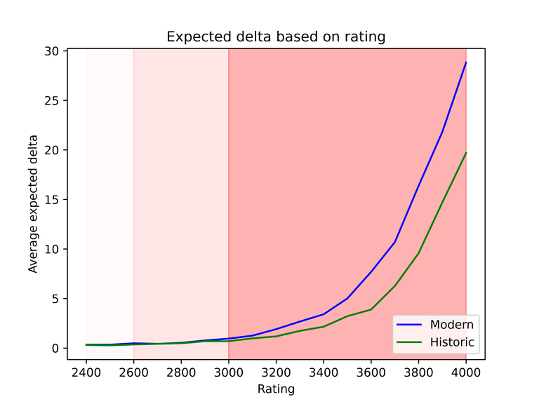
Here's your high-res graph again:

The relation is almost perfectly exponential — it turns into a line when you change the Y to a log scale. If you're 3600, you could be earning 5-10 undeserved points of delta every contest! But if you're 3000 or below, you get less than a point.

Does this actually affect us in real life?

These differences don't seem to be big enough to matter.

  • If your rating is 3500, you can maintain it with around 3480 level skill.
  • If your rating is 3400, you can maintain it with around 3385 level skill.

That seems inconsequential.

So this blog is complete cope. Unless...

Community simulation

It's possible that the high rated LGMs can pull each other up. Rating is relative — if Mike manually added 300 rating to every LGM, and they only did div0s with each other, their inflated ratings would stay.

But is this a big enough effect in practice? Could the LGMs keep their inflated ratings without leaking them back to everyone else? Let's simulate again.

Methods

We simulate all div1 players, with their ratings rounded down to the nearest 50 just to make things a bit easier. The playerbase looks like:

{3750: 1, 3700: 1, 3650: 2, 3600: 1, 3550: 2, 3500: 1, 3400: 2, 3350: 4, 3300: 3, ..., 2100: 993, 2050: 357, 2000: 531, 1950: 765, 1900: 1165}

We'll initialize each player with their real rating / their actual skill, and nominal rating / CF rating. For example, Benq becomes a Player(real_rating=3750, rating=3750).

How to simulate a the randomness in placings?

We simulated 200 trials, each of 100 contests in sequence. After each contest, nominal ratings are updated, but we assume their true ratings/skills do not change.

Results

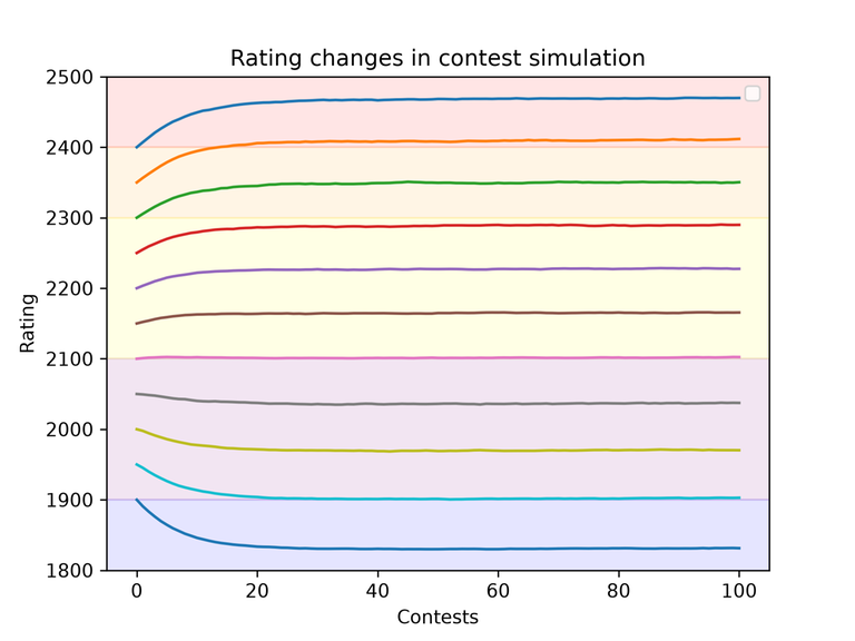
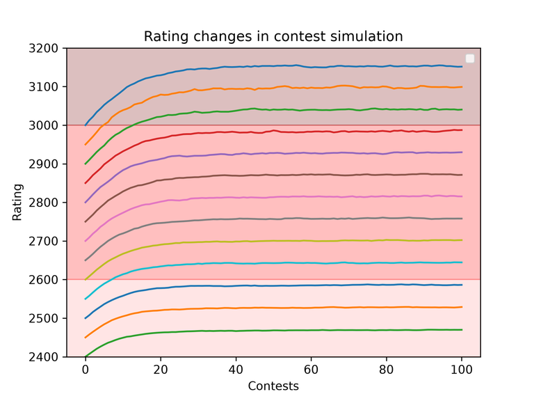
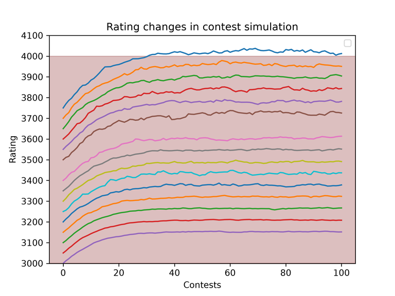
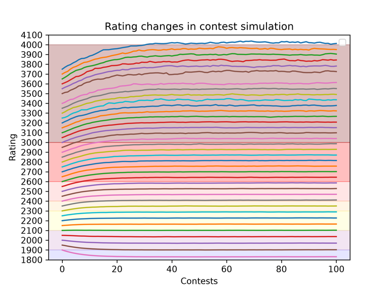
Here are the graphs:

  • 1900-2400

  • 2400-3000

  • 3000+

  • Everything

So, it seems like this is true! There is some fairly dramatic inflation at the top. And it only takes maybe 40 contests for it to fully converge. And surprisingly, it starts as early as deep red level: if your true skill is 2600, your actual rating will probably be around 2702. For LGMs, the inflation can be as high as 150-200 points.

Table of results for each rating

Is this a big problem?

Not really. It just means that the scale is a bit more stretched out than it should, especially near the top. The ratings still maintain the ability to compare.

I would assume it would also be possible to fix with some math by switching the update formula to something based on likelihood estimation. We can't simply use performance is that the performance of 1st place is infinitely large. We could do numerical max a posteriori estimation — with some rating deviation (either explicitly stored or implicitly set to, say, 100, for everyone), and we numerically update the distribution (as in, we store the distribution as a table of probability densities at, say, 0.1 rating increments) and calculate the new center (whether that be expectation, median, mode, or whatever). Also I guess calculating likelihood (which is $$$P(\text{get place 67} | \text{rating 2900})$$$) is not trivial, since you have some weird sum of Bernoulli variables.

Math rant about making the perfect system

That's it for today! As always, thanks for reading, and you can find the code and figures on my GitHub.

Full text and comments »

  • Vote: I like it
  • +211
  • Vote: I do not like it

By greateric, history, 2 months ago, In English

AHHHHHHHHHHHHHHHHHHHHHHHHHHHHHHHHHHHHHHHHHHHHHHHHHHHHHHHHHHHH 31st on div2 (and would've been 11th if i wasnt orange) and 2656 perf how is this possible i am legit shaking rn

I got to experience being on the front page for like 5 minutes and then maspy beat me ;-;

E is absolute cinema and it seems there weren't as many cheaters so that's good I guess

Also 1400 solves on D to 65 on E is crazy

On a more serious note I was getting a little depressed by round 1106 when I thought I did really well but then didn't even get orange perf. But I think this round shows that the ratings are not hopelessly deflated yet

Full text and comments »

  • Vote: I like it
  • -26
  • Vote: I do not like it

By greateric, history, 3 months ago, In English

If you were ever curious but were confused by the youtube tutorials. I'm going to try to make this as concise and useful as possible. Also, x86 is way easier to code in than ARM and if you disagree, you're wrong. And Intel syntax is better than AT&T syntax

This assumes you have a basic understanding of how pointers work in C

First program & compiling

Make a file named hello.s:

.intel_syntax noprefix

.section .rodata
mystring:
    .ascii "Hello, World!\n"
mystring_end:

.section .text
.globl main
.type main, @function
main:
    endbr64
    push rbp
    mov rbp, rsp

    mov eax, 1  # write
    mov rdi, 1  # stdout
    lea rsi, mystring[rip]
    mov rdx, mystring_end - mystring
    syscall

    xor eax, eax

    leave
    ret

Compile and run with

$ gcc -o hello hello.s
$ ./hello

In assembly, you are writing CPU instructions, so you only have access to low-level things:

  • Registers: the main ones are rax, rbx, rcx, rdx, rsi, rdi, rbp, rsp, and r8...r15
  • Memory (dereferencing pointers, writing to the stack, etc.)
  • System calls

The C stack

Your CPU only knows how to execute instructions, so how do we have functions be able to call other functions or themselves? The answer is the stack: each function has its own stack frame. For example, if main has its stack frame, and if it calls printf, then a new stack frame will be created for printf. Once printf is done executing, we will pop printf's stack frame and go back where we left off to main.

I'm now going to explain the actual nitty gritty of how this works; it may be a bit hard to follow along so if you're confused please let me know! I think it is fun to understand this though.

Two registers are dedicated to managing the stack: rbp: base pointer, and rsp: stack pointer. The base pointer points to the beginning/base of the stack frame, while the stack pointer points to the end. Also be aware that in x86, the stack grows downward, i.e., the main stack frame will be at a higher address in memory, and as more data is pushed onto the stack, the address decreases.

Here's an example of how it works in practice.

Suppose your code section looks like this (remember that code/instructions are also loaded in memory)

address instruction
main:
...
5598    load pointer corresponding to format string into rdi
55a0    load integer into rsi
55a8    call printf
55b0    set exit code to 0
55b8    leave
55c0    ret
...
printf:
57d8    endbr64
57e0    push rbp
57e8    mov rbp, rsp
57f0    random instruction that does printing
57f8    another random instruction that does printing
5800    yet another random instruction that does printing
5808    leave
5810    ret

So, we're currently on the stack frame of main() and we're about to execute the instruction call printf at 55a8. After we're done executing printf, we need to execute the instruction at 55b0. So, we push the address 55b0 onto the stack. This is called the return address, the CPU will jump to 55b0 after it's done executing printf.

Now we jump to the address of printf, 57d8. The first instruction is always endbr64, without getting too deep, it's a security feature; if you try to call a function and the first instruction is not endbr64, the CPU will segfault (if the security feature is enabled).

Then, push rbp pushes the previous (main's) base pointer to the stack. Then mov rbp, rsp makes rbp point to the beginning of the new stack frame, which is the current rsp. Note that the CPU automatically moves rsp to the end of the stack whenever anything is pushed or poped.

The stack will look something like:

address     data
7ffe6590    <random data in the stack for main, like main's local variables>
7ffe6588    <random data in the stack for main, like main's local variables>
7ffe6580    <random data in the stack for main, like main's local variables>
7ffe6578    <return address telling us where to go back to in main()>
7ffe6570    <main's rbp value saved>     # rbp now points to 7ffe6570
7ffe6568
7ffe6560
# rsp always points to the end of the stack, which is `7ffe6570` for now, but it may move down if `printf` has local variables, etc. that it wants to put on the stack.

Eventually, printf will finish executing. The leave instruction is kind of like a macro — it will dereference rbp and set rbp to that value. rbp is a pointer to the beginning of the frame but it also points to main's previous rbp value (see the figure above at 7ffe6570). So this restores rbp back to its previous value when we go back to main(). It also automatically resets the stack pointer to the beginning of the frame, which effectively "deletes" everything in the current stack frame.

Finally, ret will read the return address, which is now the last thing in the stack, and jump to the instruction we were previously at. The rbp and rsp registers are restored to the same places that they were before printf was called.

Arithmetic operations

You can perform arithmetic operations on registers. For example, add eax, ecx performs eax = eax + ecx.

Note that the letter you prefix a register with denotes its size: rax is the full 64-bit register, eax is the lower 32 bits of the register, ax is the lower 16 bits of the register, and ah is the upper byte of ax, and al is the lower byte of ax. The same thing applies for rbx, etc. For r8 through r15, it's r8 for full size, r8d for 32 bits, r8w for 16 bits, and r8b for 8 bits.

So add eax, ecx performs 32-bit addition and add rax, rcx performs 64-bit addition. For addition and subtraction, the same instruction does both signed and unsigned addition/subtraction because of some magic in the representation of integers called 2's complement.

For multiplication, it's a bit more complicated: mul rxx multiples rax by rxx and places the lower 64 bits in rax and upper 64 bits in rdx. If you do mul exx, it multiplies eax by exx and places the lower 32 bits in eax and upper 32 bits in edx.

That's unsigned multiplication. Signed multiplication is imul.

For division, it's also a little weird. div rxx takes the 128-bit value rdx:rax and divides it by rxx, places the quotient in rax and remainder in rdx. So if you want to do 64 bit division, you have to make sure to zero out rdx. Then idiv rxx is the same but for signed division. You may need to sign extend: cqo sign extends rax to rdx:rax, and cdq sign extends eax to edx:eax. (Sign extension is required if you're dealing with negative numbers.)

The multiplication and division stuff is a bit complicated, but luckily we're in the age of AI so you don't have to memorize this.

Moving data around

You've probably seen the move instruction: mov rax, rdx copies rdx into rax (and similar for 32-bit register views).

To move between registers and memory, you can do something like mov DWORD PTR [rbp-8], 572. [rbp-8] means dereference the pointer rbp-8, so we're dereferencing the location 8 bytes below the base of the current stack frame. DWORD PTR [rbp-8] means we're interpreting it as a double word (32 bits). We also have QWORD PTR (64 bits), WORD PTR (16 bits), and BYTE PTR. So this writes the number 572 into the 32-bit integer located at [rbp-8].

Here are a few more examples. Can you tell what they mean?

  1. mov eax, DWORD PTR [rbp-20]
  2. mov QWORD PTR [rbp-8], rbx
Spoiler

If you look at assembly generated by GCC, you'll see a lot of moves relative to rbp. That's because we like to reference variables by their location relative to the base of the stack frame. For example, if you declare int a, b, c; in a function, GCC may decide to place a at [rbp-4], b at [rbp-8], and c at [rbp-12].

We also have lea for load effective address. It's typically useful for pointer arithmetic (you can also just use add/sub but lea is typically more idiomatic and faster).

For example,

# This loads `rbx + rax` as an address into `rdi`. It's equivalent to `rdi = rbx + rax` so you can technically replace it with `add` instructions. In practice this could mean that `rbx` was a pointer to an array of chars and `rax` is the index, so this is `&rbx[rax]`.
# Note that we have brackets here but the memory is not actually dereferenced.
lea rdi, [rbx + rax]

# If `rbx` is a pointer to an array of 4-byte ints, then this is like `&rbx[rax]`.
# Note that you can't just put arbitrary arithmetic here, lea only allows `[base + size*index + offset]`. And size can only be 1, 2, 4, 8.
lea rdi, [rbx + 4*rax]

# If `rbx` is a pointer to 8-byte structs, and `field` is located at a 3-byte offset in the struct, then this is like `&rbx[rax].field`.
lea rdi, [rbx + 8*rax + 3]

Sections

There are .section directives. The sections are:

  • .text: code
  • .data: global variables, that can be pre-initialized to a certain value
  • .bss: global variables, that are automatically zero-initialized
  • .rodata: read-only constants, such as literal strings in C

Global variables

This in C:

int32_t y = 1000;
int64_t z = 67;
char s[] = "forcescode";

Is this in assembly:

.section .data

.globl y
y:
    # Also .byte, .short
    .long 1000

.globl z
.align 8  # Unaligned data will not cause errors in modern x86_64, but it is slower.
z:
    .quad 67

.global s
s:
    # .string or .asciz null-terminate the string, .ascii does not
    .string "forcescode"

Note that .globl is a directive for it to be visible to outside files or not. It's like static vs non-static in C.

For bss, you just reserve space:

.section .bss

.globl myarray
myarray:
    .zero 24000  # 24,000 bytes

String literals

Typically, you'll put these in rodata:

.section .rodata

mystring:
    .string "codeforces"

Also, typically when referencing data or bss values, you need instruction pointer relative addressing. Because your code needs to be position-independent, you can't have a fixed address to reference the global variable, you need it relative to rip, the instruction pointer register.

# Equivalent
lea rdi, mystring[rip]
lea rdi, [rip + mystring]

Both of these reference mystring, but as an offset relative to rip. At link time, the offset of mystring relative to rip is calculated, and then the code will correctly reference mystring.

Basic calling convention

I'll probably go in more detail on this in part 2. For now, here's the basics of how to call other functions correctly.

You pass the first 6 arguments in registers: rdi, rsi, rdx, rcx, r8, r9. The classic way to remember it is " Diana's silky dress costs 89".

Additionally, for variable argument functions like printf or scanf, you also need to zero out eax. (I'll explain why later.)

For example, if you wanted to printf("The answer is: %d\n", answer), you would

lea rdi, location_of_string[rip]  # Assuming the string literal is in .rodata
mov esi, [pointer to variable `answer`]
xor eax, eax  # "Better" way to zero out a register than `mov eax, 0`
call printf

Then, the function's return value is given in rax/eax/ax/al (depending on if the return value is a 16-bit or 32-bit or 64-bit or pointer). That's also why we do xor eax, eax at the end of main(), because that's like saying return 0.

Note that this is grossly oversimplified and that the real calling convention is a lot more complex than this. But this should be good enough for now. The other gotcha that you should know for now is that some registers may be overwritten by the function that you call, while others might not. This is called caller vs callee saved registers; for now you can assume that none of your registers are safe and to always save them to memory.

Example exercise

Write a program that reads two 32-bit signed integers from standard input, and tells tells the user "The sum of your two integers is ." Use scanf and printf from the C stdio. You do not need to worry about overflow.

How to allocate local variables, read this before attempting
Answer

In part 2, I'll probably cover more details about the calling convention (passing more arguments, structs, caller and callee saved registers) and talk about conditionals and branching. See you then!

Full text and comments »

  • Vote: I like it
  • +38
  • Vote: I do not like it

By greateric, history, 3 months ago, In English

This is the full raw recording of me virtualing the round this morning. Unfortunately I couldn't get OBS to get output my camera so I couldn't show what I was writing on my paper and it might not be as educational as I would have hoped. But maybe this will help you if you are interested in seeing how someone else thinks through a contest. Or if you're here for keyboard ASMR that's cool too.

Also for the haters. Unlike a certain other person you may know, I actually can deliver. (And not get stuck on C)

https://www.youtube.com/watch?v=B7daqwgbCqM


Also can we stop hating on comments? I swear to god if I get one more person calling me a cheater because of that. I feel like I need to add a note to my template

// This code contains comments. They were hand-inserted with love and not a result of AI-generated code.

Also also can someone please tell me how to make the chapters work? Like I think I did them correctly but they are not showing up

Full text and comments »

  • Vote: I like it
  • +31
  • Vote: I do not like it

By greateric, history, 3 months ago, In English

Hey guys it's your favorite purple not anymore CF shitposter here. We're back to hopefully non-controversial useless information lol

I think anecdotally we all have this gut feeling that it's harder to get a X perf in a div 2 than a div 3, and in turn harder to get X perf in a div 1 than a div 2. Is this urban legend or a real phenomenon?

Methodology

I took several of the most recent separated div 1 and div 2 rounds where the div 1 round has the same problems shifted by 2 positions.

For each contestant in the div 2 round, we'll:

  • Calculate and record their div 2 perf
  • Convert to estimated div 1 score by dropping problem A/B, adjusting timestamps on the rest of the problems, and recalculating the score based on the problem values for div 1. (We will discard anyone who solves C/D/E/F before A/B)
  • Calculate and record their div 1 perf from the new score we calculate.

Calculating performance (CP lesson time!)

Using FFT, our favorite :yayy:

Let's formally define performance as, position $$$p$$$ having performance $$$x$$$ means that if your rating was $$$x$$$, then the expected value of your placing is $$$p$$$.

If we make places 0-based (winning would be 0th place), we can use linearity of expectation:

$$$E[\text{place}] = E[\text{tourist}] + E[\text{Benq}] + ... + E[\text{greateric}] + ... + E[\text{another random person}],$$$

where $$$E[\text{tourist}]$$$ is the chance of you losing to tourist, which is given by

$$$\displaystyle \frac{1}{1 + e^{(x-y)/173.7178}},$$$

where $$$y$$$ is the rating of the other participant and $$$x$$$ is the performance.

This is how Codeforces (and we) will calculate the performance.

Now the fun part is that we can speed this up using FFT. Instead of having an quadratic-type algorithm where you have to spend $$$O(n)$$$ time summing up all those expectations for every performance you want to calculate, let's convolve them.

Define a one-hot encoding array $$$a$$$ such that $$$a_i$$$ is the number of people in the field with rating $$$i$$$. For example, if there are 2 people with rating 3 and 1 person with rating 4, we might have $$$a = [0, 0, 2, 1, 0]$$$.

Then, the place of a performance $$$x$$$, which I will call $$$f(x)$$$, is:

$$$\displaystyle a_1 \cdot \frac{1}{1 + e^{(x-1)/173.7178}} + a_2 \cdot \frac{1}{1 + e^{(x-2)/173.7178}} + ...$$$

Do you see the convolution/cross-correlation yet? We essentially want to convolve an array $$$b$$$ that contains all the lose-chances in a sliding window along the array $$$a$$$. That would calculate all the performances of all the ratings in a range $$$[l, r]$$$ in time $$$(r-l) \log (r-l)$$$.


Here's an illustration to try to show this more concretely. Let's assume that in this fictional rating system, you trade games when your rating is equal, have a 70% chance to win if your rating is 1 point higher, and are guaranteed to win if your rating is 2 or more points higher. In other words, $$$b$$$ would look like $$$[..., 0, 0, 0.3, 0.5, 0.7, 1, 1, ...]$$$

Then suppose our one-hot is $$$a = [1, 0, 0, 1, 2]$$$: 1 person with rating 1, 1 person with rating 4, 2 people with rating 5. We would calculate:

rating       1    2    3    4    5
    a        1    0    0    1    2
       0.3  0.5  0.7   1    1    1    1     # suppose our rating is 1

# Expected placing: 1*0.5 + 0*0.7 + 0*1 + 1*1 + 2*1 = 3.5
# So placing 3.5 would be a performance of 1 rating.

rating       1    2    3    4    5
    a        1    0    0    1    2
            0.3  0.5  0.7   1    1    1     # suppose our rating is 2 now

# Expected placing: 1*0.3 + 0*0.5 + 0*0.7 + 1*1 + 2*1 = 3.3
# So placing 3.3 would be a performance of 2 rating.

# And so on, moving the window

Once we have that, we take the time spent to solve div 2 C/D/E/... and map that to div 1 A/B/C. This allows us to calculate the score and performance in the div 1 round.

Results

I analyzed all 15 div 1/2 separated rounds over roughly the last year. The results are... weird.

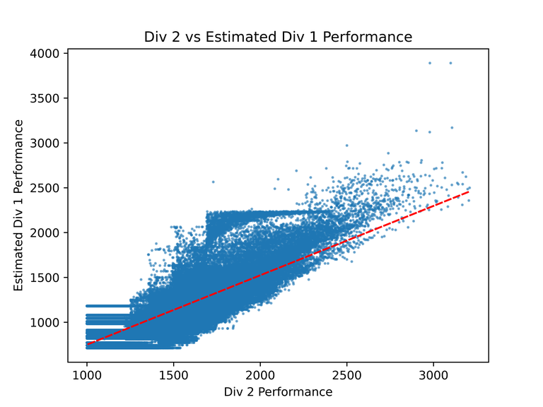
This is the graph of div 2 vs div 1 performance over them all.

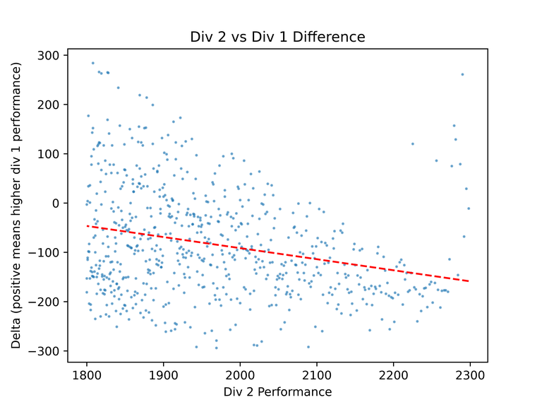
For the most recent round 1105, for most people in the 1800 to 2300 range, div 1 was roughly 50 to 120 rating points harder.

However, over all rounds, div 1 was approximately 400 points harder than div 2. There was a lot of variance between rounds; some had div 1s up to 600 points harder, and others had div 1s that were actually a few points easier. This doesn't really make a lot of sense; intuitively we all know that can't be true.

Some explanations for the somewhat crazy results could include:

  • You do lose the time you spent on div 2 A/B into a black hole forever. Even if we adjust the penalty, you may lose the ability to solve an additional problem if you just needed another like 5 or 10 minutes of time.
  • You are "fresher" in div 1, since you don't have to spend any mental energy on div 2 A/B.
  • There could be some bias in the data. Maybe a lot of people who "place well but not too well" in div 2 were boosted by really fast/accurate solves on div 2 A/B that go away when we remove them in div 1. For example for most people in the 1600-2000 perf range their div 1 data is really only the time it took them to solve problem C after B, or to solve problems C and D. It is also possible that div 1 rewards solves on harder problems more than speed on early problems.
  • "Unregister scumming." Basically you read problem A (maybe also B) and try to solve it in your head, if you don't get the idea fast enough then you just give up and unregister. You don't become committed to the round until you send your first submission. Unregister scumming is much more effective in div 1 because the first problem is already decently hard — I could unregister scum in div 1 fairly effectively, in the contests where I get a fast solve on A I'd be at a sizable advantage, or I could quit if the problem looks like implementation hell, WA hell, or something like that. On the other hand, if I tried to unregister scum in div 2 it would be way harder since problem A will always be a fast solve to me anyway.
  • Maybe my method is just bugged?
  • Or div 1 could really be deflated by that much in comparison to div 2.

If you were hoping for a number with a nice-looking confidence interval attached, sorry! Unfortunately this data is not nice to work with. You can find the rest of the high-res graphs for each contest at https://github.com/greatericontop/Codeforces-Div1vsDiv2/tree/main/assets/per_contest. You can also get the source code there and run some tests yourself and/or potentially find a bug in my approach that might be causing the results lol

Why do ratings desync?

Ratings can only compare skill across a population if the entire population interacts. Otherwise, such as in the case of div 1 and div 2, you may end up with "div 1 flavored rating" and "div 2 flavored rating" that cannot be compared to each other.

The solution is to make sure the populations mix as much as possible. I think CF does a pretty decent job at this. We have combined 1+2 rounds every so often that mix everyone together, and div 3/4 participants can also participate in div 2 which does some mixing there.

A quick note on problem ratings

You may also have a gut feeling that a 2100-rated div 3/4 problem is easier than a 2100-rated div 1/2 problem.

I think this is true given what we know about div 1 vs div 2 flavored ratings. What also could be a factor is positioning — a div 3 F may be the same difficulty as a div 2 D, but div 3 contestants had less time during the contest to solve it on average. That can artificially drive up the rating of the div 3 problem.

Full text and comments »

  • Vote: I like it
  • +55
  • Vote: I do not like it

By greateric, history, 3 months ago, In English

Background

On CF I think you can tend to see people attributing good rating to IQ. This is often associated with hopelessness when people are stuck in gray/green.

I think it's the perfect cope — it's the easiest thing to say that completely explains why you're 1100 and your friend is orange, and, bonus, if anyone tries to prove you wrong, you can just claim that they are privileged and intelligent.

You may think I am 2000 and thus out of touch to be able to comment on this topic, which may be true. However, I was also once a noob who got 28/1000 on a USACO silver round. And I was pretty overweight as a kid and sucked at sports and always thought of myself as not having the genetics to be an athlete, but I now hold the squat, bench, and deadlift 18-and-under state records in my powerlifting federation. (Probably not for long though lol)

A lot of this is inspired by my powerlifting coach, Matt Vena. He's big on psychology in sport and I think that has greatly improved my progress in both powerlifting and CP. Also that's why a lot of my examples are lifting related

Self-limiting beliefs influence results

Your beliefs can improve or harm your progress. Simply being told that you have good IQ for CP or good genetics for powerlifting can impact your abilities.

  1. Male varsity athletes were given placebo steroids. On bench and squat, placebo steroids resulted in significantly higher strength gains (p < 0.05 on an F-test), while on the other two exercises the difference was not significant. (Ariel & Saville, 1972)
  2. Nationally ranked powerlifters were given fake steroids and improved their totals by around 70 pounds instantly when told they were given steroids. For reference, I would be super happy with a 70 pound increase in my total in 4 months. (Maganaris, 2000; analysis by Greg Nuckols from Stronger by Science) The funniest part is that when they told half of the lifters that the steroids were fake, they immediately lost the "fake strength" they had gained!
  3. They measured a gene associated with aerobic capacity (how fast you can run), and told half the participants the truth and lied to the other half. Being told that one had the good gene had a greater effect size than actually having the good gene! (Turnwald et al., 2019; analysis by Greg Nuckols from Stronger by Science)
  4. In the famous "Mind over Milkshake" study, hormonal hunger responses to food were affected by whether the milkshake was labeled low or high calories, even though all of them actually had the same amount. (Crum et al., 2011)

Bonus resource: another Stronger by Science article.

The bottom line is, if your expectations can so greatly influence inherently physiological things like strength, mile time, or hunger horomone levels, how greatly can they influence a mind sport like CP?

Worry about what you can control

Let's abstractly model

$$$\text{CF Rating} = \text{IQ} + \text{Work},$$$
$$$\text{Weight Lifted} = \text{Genetics} + \text{Work},$$$

where $$$\text{Work}$$$ is a combination of good coaching, effort put into practice every day, and additionally for powerlifting things like sleep, nutrition, etc.

I won't pretend like I have data to support this, but for most people the $$$\text{Work}$$$ value will quickly outpace the $$$\text{IQ}$$$ value. Low effort practice for not a long time may be something like 1000 if your genetics/IQ is unlucky to 1700 if it is. With lots of high effort over a long period of time, even if you are unlucky, I think you can reach 2200 or 2300 eventually, and if you are lucky then you will become tourist.

Anecdotally, I also have noticed that a lot of powerlifting champions come from the same area. (For those into powerlifting, take for example Dillon Johnson and Chase Gravitt being from the same gym, lots of people at PWRBLD, Will Ball literally training in Evan Hawk's living room, etc.) If genetics mattered a lot more than effort, we should expect high-level lifters randomly distributed across the country. Instead, we see a boost in results that is probably caused by a boost in effort from having multiple high-level lifters motivating each other.

Again, I'm not going to pretend that this is scientifically supported data, but whenever I'm at the gym, I tend to notice that the people with the biggest muscles are also the ones that show up every day and hit the workouts that they have planned. Also among my friends I can pretty easily see who will improve and who won't depending on how seriously they take the sport.

IQ is a shit metric anyway

If you're still not convinced that IQ and genetics are cope, an IQ test is a horrifically bad indicator of intelligence. It only really captures how good you are at something at the very moment, not how good you can get over time.

You may say that you're not meant to be able to get better at IQ tests

They can't even measure intelligence. Some guy DMed me a few weeks ago asking me to take a CORE IQ test, and they have you do:

Algebra on shapes in your head
Memorizing digits

If there are some other ones you want to see me debunk, let me know.

And how do you make sure an IQ test is measuring intelligence, which I'm defining here as similar to genetics, which is something that you're born with? And not something that is practiceable, like shapes-on-scales algebra, pattern recognition in competitive programming, or digit memorizing? If you're going to give up after seeing a test result, it should be seeing the rating you can reach, not what is essentially a heavily confounded measurement of your rating right now.

But this IQ test has WXYZ r^2 value correlation with SAT score / math rating / CF rating!

You're more average than you think

What if I told you that you could be the a GM with some practice?

You'd probably say, nah, I'm not lucky enough to be one of those people.

Then why do you think you're unlucky enough to be stuck in newbie forever?

The population average is the average for a reason. You're probably there.

So why aren't you improving?

Proper methods

"Just practice more" is not optimal advice in my opinion. If you're doing English problems to practice CP, that's obviously not going to get you very far.

Read up on how a bunch of accomplished people like to practice, and also be introspective about your own practice. Try to identify weaknesses to work on, what things you do that seem to work well, etc.

Remember that there are multiple optimal approaches to training; as long as you're following the general principles, you will be okay.

Self-deception

It's easy to think you are putting a very high amount of effort when you are actually half-assing it every day. Refer to https://codeforces.me/blog/entry/98621 .

Time

If you think you can go from 1400 to 2000 in a month practicing an hour per day, then that would imply that I could go from 2000 to something like 2900 in a year practicing 3 hours per day.

Once you get out of the beginner stage, the amount of time it takes to notice improvement will start to be measured in months. In powerlifting, I do a 4-month training cycle and then compete at the end. On a good training cycle, I'll be able to add something like 17.5 kilos to my squat. That's less than 10 pounds per month, and that's with powerlifting taking up a significant chunk of my life (I spend about 13 hours per week in the gym, another like 2 hours of cardio now every week, and nutrition and sleep).

Okay, but what if I'm actually stupid?

If you can:

  • Understand the tutorials and most (like 80-90%) of the editorials of easy/normal problems and some of the hard problems on USACO Guide silver section, and maybe also the gold section if you want to get beyond ~1800ish(?) (very rough estimate and my opinion only)
  • Notice yourself applying a technique you learned from a past problem every so often. (It does not have to be every problem, I'll only think "oh hey this problem uses a strat I have kind of used before" maybe once every like 15 problems.)
  • If you get stuck on a problem that's like within 300 points above your rating and read the editorial, you should be able to understand the editorial solution most of the time. (It is ok to spend a while to digest the editorial, or not understand it entirely every so often.)

Then you're at where I am and you're probably smart enough. Put in some hours — genuine hours, but also intelligently allocated hours — and I'm sure you'll improve.

Also read Zhtluo's blog on being Russian. "I think I'm stupid and low IQ, the trick looks obvious" may be the emotion you feel when it's actually "I haven't done enough CP to be good at the 'Russianness' ability to spot tricks/strategies". The trick for most 1400-1700 problems, even into the 2000s, are always obvious in hindsight; try your best to not feel too bad if you fail to see what you think should have been obvious (obviously it is ok to be disappointed... I feel it too) (but now you will never make that mistake ever again!)

Extra extra bonus tip (secret)


To recap:

  • Expectations matter. Your overstressing about IQ hurts you more than having an allegedly bad IQ.
  • Effort outperforms IQ/genetics. (Anecdotally)
  • IQ tests aren't good statistical tools.
  • Your IQ/genetics are probably average.

So yeah, that's my rant for the day. More technical posts will be back $$$\text{Soon}^\text{TM}$$$.

If you want to argue with me in the comments (and/or increase the absolute value of my contribution by turning it negative), please do (actually please don't turn my contribution negative); I'll try to keep an open mind.

Full text and comments »

  • Vote: I like it
  • +67
  • Vote: I do not like it

By greateric, history, 3 months ago, In English

Don't worry, your regularly scheduled useless information programming will resume soon.

Anyway, here is gtest, my attempt at writing a script to help with stresstesting.

Note that I still personally think stresstesting is slightly overrated. It is not a silver bullet, especially when some questions are unstresstestable, like some constructive problems, problems where the solution space grows way faster than even exponentially if you're trying to brute, other cases where your brute forcer has to make some core observation that could potentially be wrong, or if your brute forcer is bugged too and misses the same edge case your fast solution does (Cirno and Number with digit 0 be like). I also think it takes a lot of time so you decide whether you want to write everything up or not. With that being said though, it should be very helpful for debugging WA2s, hopefully.

The format is

gtest -s <path to solution 1> -t <path to solution 2> -g <path to generator> [-c <path to checker>] [-T <trials>]

It supports:

  • Custom checker (the default just compares the tokens in the two outputted solutions). Also, the -t argument is optional, since for some constructive problems maybe you just want to code your solution and a checker that confirms your solution is correct.
  • Solutions, checkers, and generators can be written in Python or C++ (I didn't add support for any other languages sorry lol)

Example:

Solutions

Literally just drop your current solution (.cpp will be compiled automatically; .py will be run with python automatically; executables will be run by themselves) in. And code your brute force solution the same way since they'll be reading the same input.

In the example, we have two solutions for two sum on the same input format (n on one line, target on the next, then the array).

Using checkers

The two solutions' standard outputs are redirected to 1.out and 2.out so go ahead and open those files and see. You should return exit code 0 to give AC and exit code nonzero to give WA. For an example, see token_checker() in gtest.py.

Using generators

For C++ generators, just write your test data to stdout, it will be redirected. Seed your RNG as appropriate.

For Python generators, the script will load the module (using importlib) and extract every function you write that starts with gen_. So you can write multiple generators, like gen_small(), gen_medium(), gen_maximum() and it will run all of them. Again, just write to stdout (such as with print), it will be redirected.

Installation

Go here https://github.com/greatericontop/gtest, clone the repo, and run make install. Alternatively just copy the python script gtest.py and put it somewhere. It has no dependencies other than python STL.

I didn't see a lot of good stresstesting tools publicly available. Hopefully this is useful!

Example usage

Here is what I did while debugging a WA25 (actual hell) on 1808C. (Read the problem first so the code makes more sense)

First I write a super stupid brute forcer:

t = int(input())
for tt in range(t):
    left, right = map(int, input().split())
    best_luckiness = 1000
    which_num = None
    for i in range(left, right + 1):
        s = [c for c in str(i)]
        s.sort()
        luckiness = int(s[-1]) - int(s[0])
        if luckiness < best_luckiness:
            best_luckiness = luckiness
            which_num = i
    print(which_num)

And a few generators:

def gen_borderline_interval():
    left = randint(10**18 - 500, 10**18)
    right = left + randint(1, 500)
    right = min(right, MAX)
    print(1)
    print(left, right)

def gen_tiny_interval():
    left = randint(1, 10)
    right = left + randint(0, 10)
    right = min(right, MAX)
    print(1)
    print(left, right)

This problem requires a custom checker since the answers generated by the two solutions may not actually be the same:

# Checker should read the input and both solution outputs manually
with open('gen.in', 'r') as f:
    f.readline()
    left, right = map(int, f.readline().split())
with open('1.out', 'r') as f:
    ans1 = int(f.readline().strip())  # In this case I hardcoded it to only check 1 case, which is fine, you don't need it to be beautiful
with open('2.out', 'r') as f:
    ans2 = int(f.readline().strip())

s1 = [int(c) for c in str(ans1)]
s2 = [int(c) for c in str(ans2)]
l1 = max(s1) - min(s1)
l2 = max(s2) - min(s2)
assert left <= ans1 <= right  # A tripped assert will exit non-zero and thus be interpreted as WA
assert left <= ans2 <= right
if l1 != l2:
    print('WA luckinesses are different')
    exit(10)

A few hundred runs later, I find out that I'm kind of stupid:

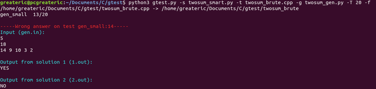
$ gtest -s 1808C -t 1808C.py -g 1808C_gen.py -T 2000 -f -c 1808C_checker.py
gen_borderline_interval  175/2000Traceback (most recent call last):
  File ..., in <module>
    assert left <= ans1 <= right
AssertionError


-----Wrong answer on test gen_borderline_interval:176-----
Input (gen.in):
1
1000000000000000000 1000000000000000000

Output from solution 1 (1.out):
1

Output from solution 2 (2.out):
1000000000000000000

Took me about 8 minutes to write the brute, generator, and checker, so not too bad in terms of time in my opinion.

Full text and comments »

  • Vote: I like it
  • +22
  • Vote: I do not like it

By greateric, history, 3 months ago, In English

part 2 to farm contribution ahahahahahahaha

Mathematical definition of Elo

Elo is intended to measure skill. Formally, skill is how likely you are to win a game (we're still focusing on two-player for now). If a player with a high rating plays against a player with a low rating, we would expect the higher rated player to win more, on average.

Now let's define what rating is. If player A has rating $$$a$$$ and player B has rating $$$b$$$, then player A should have a $$$\sigma(\frac{a-b}{\beta})$$$, where $$$\beta = \frac{400}{\ln 10} = 173.7178$$$, and $$$\sigma()$$$ is the sigmoid function $$$\sigma(z) = \frac{1}{1+e^{-z}}$$$.

This formula looks scary, but it's just a formal way of writing the one you might be familiar with. This formula expands/simplifies to:

$$$\frac{1}{1 + e^{-\frac{a-b}{400 / \ln 10}}}$$$
$$$= \frac{1}{1 + 10^{\frac{b-a}{400}}}.$$$

You're probably more familiar with the last equation above. If you are 400 points weaker, you'd have a 1 to 10 ($$$\frac{1}{11}$$$) chance of winning; if you are 800 points weaker, you'd have a 1 to 100 ($$$\frac{1}{101}$$$) chance of winning.

Elo sucks

A good rating system should have good success at prediction on a dataset. Elo is... not good at that. It only maintains a single rating value for each player. A GM who starts at 1500 may have to win many games to get their rating up to the 2000s, and a bad player may have to slog through like 15 full games of getting destroyed by strong opponents before they finally find their rating.

Heuristically, new players' ratings should probably change faster, and they shouldn't change their opponents' ratings as much (since we are not very confident about their true skill).

"Confident"... yes, this is a job for statistics :yayy:

Modeling ratings as priors and posteriors

We have an initial belief about a player's skill level. Our first improvement will be as follows: instead of having only the rating, we will have the rating and rating deviation (RD). Essentially, we are regarding a player's true rating as an unknown variable, but we have an estimate for it in the form of a normal distribution with mean equal to the rating and standard deviation equal to the RD.

Now, we will use Bayesian likelihood estimation to update our old distribution into a new distribution (new rating and RD) with the information from the result of a game.

Get ready for some math!

We want to update our (we will update one player at a time for now) rating. Assume we start with rating $$$0$$$ for simplicity (just subtract $$$a$$$ from both sides), and our opponent has rating $$$\mu_y$$$ ($$$\mu_y=b-a$$$). Our RD is $$$\sigma_x$$$ and their RD is $$$\sigma_y$$$. Suppose we win the game.

Likelihood

What is the likelihood we win? Suppose we knew with certainty that our rating was exactly $$$x$$$ ($$$x$$$ does not have to be zero), and our opponent's rating is exactly $$$y$$$.

Then the chance that we win this game is just $$$\sigma\left(\frac{x-y}{\beta}\right)$$$.

Now let's assume that we know with certainty that our rating is exactly $$$x$$$. However, we don't know $$$y$$$, only that it's drawn from the normal distribution $$$\mu_y, \sigma_y$$$.

So we need to calculate the expectation of the likelihood $$$\sigma\left(\frac{x-y}{\beta}\right)$$$ integrated over all $$$y$$$.

This is given by

$$$L(x) = \mathbb{E}_y\left[ \sigma\left(\frac{x-y}{\beta}\right) \right] = \displaystyle\int_{-\infty}^{+\infty} \operatorname{normalpdf}(y) \cdot \sigma\left(\frac{x-y}{\beta}\right) \space dy.$$$

This integral has no solution, but can be approximated very well by:

$$$g = \sqrt{ \beta^2 + \frac{\pi}{8} \sigma_y^2 },$$$
$$$L(x) = \sigma\left(\frac{x-\mu_y}{g}\right).$$$

Here is a link to a derivation of this. I don't understand it though lol

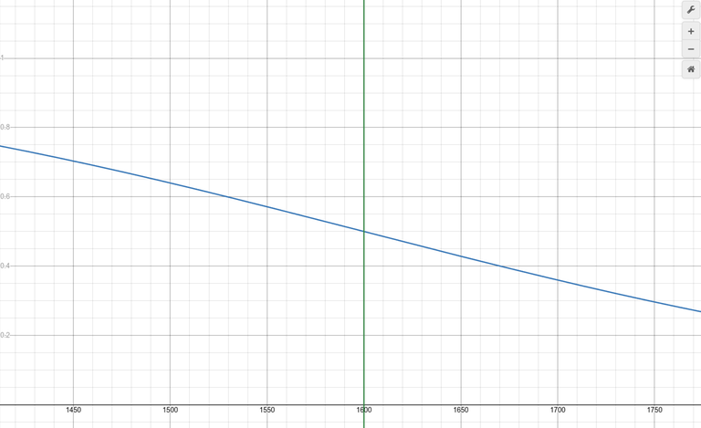
You can play around and see how good the approximation is on this Desmos graph

Posterior distribution

Now let's use our formula

$$$\text{Posterior} = \text{Likelihood} \cdot \text{Prior},$$$
$$$P(x) = \sigma\left(\frac{x-\mu_y}{g}\right) \cdot \operatorname{npdf}\left(\frac{x}{\sigma_x}\right),$$$

where $$$\operatorname{npdf}(z)$$$ is the standard normal PDF (the probability density when you are $$$z$$$ standard deviations from the mean). The prior distribution for $$$x$$$ is centered at mean 0 with standard deviation $$$\sigma_x$$$ and thus has PDF given by $$$\operatorname{npdf}\left(\frac{x}{\sigma_x}\right)$$$.

Note that $$$P(x)$$$ is technically not a valid PDF until we normalize it and make its integral equal to 1, but that's not super important to us here.

Laplace approximation

This PDF is not normal, but it turns out it is close enough (ish) in practice that we can perform a Laplace approximation. Given a PDF, this lets us approximate it as a normal distribution by:

Mean

The estimated mean is the mode of the PDF. To find the mode of the PDF, we do derivative optimization to find the maximum of the PDF. Specifically, let's optimize $$$\ln P(x)$$$ instead.

$$$\displaystyle \ln P(x) = \ln \sigma\left(\frac{x-\mu_y}{g}\right) + \ln \operatorname{npdf}\left(\frac{x}{\sigma_x}\right),$$$
$$$\displaystyle \ln P(x) = \ln \sigma\left(\frac{x-\mu_y}{g}\right) - \frac{x^2}{2\sigma_x^2} + \ln\left(\frac{1}{\sqrt{2\pi}}\right),$$$
$$$\displaystyle \left(\ln P(x)\right)' = 0 = \frac{1 - \sigma\left(\frac{x-\mu_y}{g}\right)}{g} - \frac{x}{\sigma_x^2},$$$
$$$\displaystyle \frac{1 - \sigma\left(\frac{x-\mu_y}{g}\right)}{g} = \frac{x}{\sigma_x^2}.$$$

In order to solve this for for $$$x$$$, we can either

  • use a linear approximation for $$$\sigma()$$$ and then solve analytically, or
  • for better accuracy, use a higher degree polynomial approximation, or use numerical methods like Newton's method or binary/ternary search.

For now, I'll show you the linear approximation (technically quadratic, since the coefficient for the squared term is zero) method $$$\sigma(z) \approx \frac{1}{2} + \frac{1}{4}z$$$, but be aware that it does start giving questionable results when the difference in ratings of the two players is very large.

$$$\displaystyle 1 - \left( \frac{1}{2} + \frac{x-\mu_y}{4g} \right) = \frac{xg}{\sigma_x^2},$$$
$$$\displaystyle \overline{x} = \frac{ \frac{1}{2} + \frac{\mu_y}{4g} }{ \frac{g}{\sigma_x^2} + \frac{1}{4g} }.$$$

Variance/standard deviation

Let's calculate the precision, which is equal to the negative second derivative of the log PDF evaluated at our new estimate $$$\overline{x}$$$.

$$$p = -(\ln P(x))' '$$$
$$$\displaystyle p = -\left[ \frac{ - \sigma\left(\frac{\overline x}{g}\right) \left(1 - \sigma\left(\frac{\overline x}{g}\right)\right) }{g^2} - \frac{1}{\sigma_x^2} \right],$$$
$$$\displaystyle p = \frac{ \sigma\left(\frac{\overline x}{g}\right) \left(1 - \sigma\left(\frac{\overline x}{g}\right)\right) }{g^2} + \frac{1}{\sigma_x^2}.$$$

Then the new standard deviation is $$$p^{-1/2}$$$.

$$$\displaystyle \sigma_{new} = \left[ \frac{ \sigma\left(\frac{\overline x}{g}\right) \left(1 - \sigma\left(\frac{\overline x}{g}\right)\right) }{g^2} + \frac{1}{\sigma_x^2} \right]^{-\frac{1}{2}}.$$$

Conclusion

And there you have it! That is how to update the rating and RD of a player. Remember that $$$\overline x$$$ is the new rating if the old rating was $$$0$$$, so it's actually the rating delta in this case. You'd repeat the same thing for the opponent who lost. It turns out that when you lose, the formulas are just the same, you just subtract $$$\overline x$$$ instead of adding it for the winning player.

You can see a visualization of how good the Laplace approximation is compared to the actual PDF in this Desmos calculator. You'll see that the approximation is very strong when $$$\mu_y$$$ is small, and also when $$$\sigma_x$$$ is small — but when $$$\sigma_x$$$ is large the approximation only drifts off a little bit, but when $$$\mu_y$$$ is very negative you might lose rating from winning a game...

However, if you try using a constant approximation:

$$$\displaystyle \sigma\left(\frac{x-\mu_y}{g}\right) \approx \sigma\left(-\frac{\mu_y}{g}\right),$$$

you get the update formula

$$$\displaystyle x = \frac{\sigma_x^2}{g} \cdot \left(1 - \sigma\left(-\frac{\mu_y}{g}\right)\right),$$$

which does work much better for very negative $$$\mu_y$$$, but is slightly worse everywhere else. Probably the best approach is a hybrid approach: use a linear approximation, but use a Taylor polynomial centered at $$$-\frac{\mu_y}{g}$$$ instead of always centering it at zero. But that gets deep into notation hell and I'm lazy.

Otherwise, this is a rating system derived entirely from statistics! If you read Mark Glickman's Glicko paper, you may notice a lot of similarities with mine, since they're both based on similar ideas (each player is modeled by a normal distribution, Elo-style sigmoid likelihood). If you have any questions, please ask! (or tell me if I made a mistake lol)

I have used this system on my minecraft server to great success :)

(yes i made lgm 2600 what are you gonna do about it)

Full text and comments »

  • Vote: I like it
  • +58
  • Vote: I do not like it

By greateric, history, 3 months ago, In English

(this might be a 2 parter because way too much math lol)

How do you design a good rating system? (focusing on 2-player games here, not CF)

Conditional probability primer

Suppose I have access to two coins.

  • Coin A: is a fair coin, lands heads or tails with 50% probability
  • Coin B: is heads on both sides coin, lands heads or heads with 50% probability

I choose one of them uniformly at random, flip it, and tell you I got heads. What's the chance I picked coin A and coin B, given that I got heads?

You can imagine 4 possible worlds, all with 25% chance of occurring:

  • Coin A, lands heads (1)
  • Coin A, lands tails (2)
  • Coin B, lands heads (3)
  • Coin B, lands heads (4)

We're told we can be in world (1), (3), or (4), so there's a $$$\frac{1}{3}$$$ chance we picked coin A and a $$$\frac{2}{3}$$$ chance that we picked coin B.

We write the probability of $$$A$$$ happening given event $$$B$$$ happened as $$$P(A | B)$$$.

The chance of $$$A$$$ happening given event $$$B$$$ happened is:

  • $$$P(A \wedge B)$$$ — all the worlds where $$$A$$$ happened, but you can only count the ones where $$$B$$$ also happened, which is in our case (1) if you're after the first coin, or (3) and (4) if you're after the second coin.
  • Divided by $$$P(B)$$$ — all the worlds where $$$B$$$ happened, which is in our case (1), (3), and (4), or 75%.

Bayes' Theorem

With some simple algebraic manipulation you can get

$$$P(A | B) = \frac{P(B|A) P(A)}{P(B)}.$$$

You can use this to do the famous disease testing "paradox". Suppose 1 in 1,000 people are infected with a disease $$$P(d) = 0.001$$$. Suppose you have a test that is 99% accurate: $$$P(+ | d) = 0.99, P(- | nod) = 0.99$$$.

Then we have $$$P(+) = P(+ | d) P(d) + P(+ | nod) P(nod) = (0.99)(0.001) + (0.01)(0.999) = 0.01098$$$.

And by Bayes' Theorem, if you test positive for the disease, you only actually have a

$$$P(d | +) = \frac{P(+ | d) P(d)}{P(+)} = \frac{0.99 \cdot 0.001}{0.01098} = 0.0902$$$

chance of having the disease.

Bayesian Likelihood Estimation

Consider a scenario where I have picked a coin with probability $$$p$$$ of being heads. You're told that $$$0 \le p \le 1$$$, and that $$$p$$$ is chosen in increments of 10%, so the only possible values are $$$0, 0.1, 0.2, ..., 0.9, 1$$$.

Initially, I tell you that I have chosen the value of $$$p$$$ out of all 11 possible choices with equal probability.

Now I flip the coin and it lands heads. This gives you more information — now you know it's probably more likely I chose a higher value of $$$p$$$. Can we quantify this?

The below illustration is simply an illustration — it's not perfectly rigorous but should hopefully be helpful for building intuition when I give you the formula later.

Consider $$$1{,}100$$$ worlds:

  • $$$100$$$ worlds where $$$p=0$$$
  • $$$100$$$ worlds where $$$p=0.1$$$
  • ...
  • $$$100$$$ worlds where $$$p=1$$$

Then,

  • $$$0$$$ of $$$100$$$ worlds where $$$p=0$$$ will land heads
  • $$$10$$$ of $$$100$$$ worlds where $$$p=0.1$$$ will land heads
  • ...
  • $$$100$$$ of $$$100$$$ worlds where $$$p=1$$$ will land heads

Therefore, there are $$$550$$$ worlds where the coin lands heads. We're told we are in one of these $$$550$$$ worlds, so, for example, the chance of $$$p=0.1$$$ is $$$\frac{10}{550}$$$ and the chance of $$$p=1$$$ is $$$\frac{100}{550}$$$. You can see how higher values of $$$p$$$ are much more likely.

Okay, now let's formalize it.

We're trying to estimate an unknown parameter $$$\theta$$$. It could be a probability, a mean, etc.

Our prior is our initial belief about the parameter $$$\theta$$$. In our example above, it's a discrete probability distribution with $$$\frac{1}{11}$$$ chance for each of $$$0, 0.1, ..., 1$$$. The probability distribution could also be continuous.

Our likelihood is the chance that, given a specific value of $$$\theta$$$, we get the outcome that we observed. For example, if we observe heads in the above example, the likelihood of observing heads with $$$p=0.4$$$ is 0.4. The likelihood of observing heads with $$$p=0.8$$$ is 0.8.

Finally, we should end up with the posterior — the new, updated probability distribution of our belief about $$$\theta$$$. In our case, that was the chance of $$$p=0.1$$$ being $$$\frac{10}{550}$$$, etc.

The formula is:

$$$\text{Posterior} = \text{Likelihood} \cdot \text{Prior}.$$$

(You do have to divide by the appropriate normalizing constant to make the integral of the posterior's probability density/mass function equal to 1.) When I write multiplication, I literally mean pointwise multiplication.

For instance, in the previous example with $$$p=0.1$$$, the prior is $$$\frac{1}{11}$$$, the likelihood is $$$\frac{1}{10}$$$, so the posterior is proportional to $$$\frac{1}{110}$$$. This is a factor of $$$2$$$ below the actual value we calculated, but that's because we have to divide by the normalizing constant which is the overall likelihood (it's like dividing by $$$P(B)$$$ at the bottom of Bayes' Theorem) (in fact it's literally just Bayes' Theorem, the prior is like $$$P(A)$$$, and the likelihood is $$$P(B | A)$$$), $$$\frac{1}{2}$$$ in this case.

As you can see, this method of inference is very powerful — you can continually update your beliefs about a hidden variable as more information comes in. You can use this in chess rating systems, exposing Dream for cheating for the 676767677th time, and also AI (because machine learning is just glorified statistics let's be fr)

Anyway I think that's enough math for today and I'll make a post over how to use this to create a rating system later (tomorrow?)

Full text and comments »

  • Vote: I like it
  • +21
  • Vote: I do not like it

By greateric, history, 3 months ago, In English

I'm writing this while there's a tornado warning at Purdue but I refuse to die until I reach orange

Wanted to share an idea that comes up reasonably often in my opinion. Essentially, you can take advantage of some property of the minimum or maximum of an array or some other structure to construct/calculate the answer starting from there.

2129B/2130D — Difficulty: 1600

Hint 1
Hint 2
Hint 3
Answer

2067D — Difficulty: 1900

Hint 1
Hint 2
Hint 3
Hint 4
Hint 5
Hint 6
Hint 7
Answer

1852B/1853D — Difficulty: 1800 on CF, 2000 on CList, definitely feels more like a 2000 to me

Hint 1
Hint 2
Hint 3
Hint 4
Hint 5
Hint 6
Answer

2234E (just 2 contests ago!) — Difficulty: 2100

Hint 1
Hint 2
Hint 3
Hint 4
Hint 5
Hint 6
Answer

How do I get better at spotting this?

Probably just practice! You'll start to remember to think about it more often and start seeing the patterns like this one.

Full text and comments »

  • Vote: I like it
  • +37
  • Vote: I do not like it

By greateric, history, 3 months ago, In English

In practice our C++ solutions get to be run with Undefined Behavior Sanitizer, also known as the diagnostics, which catch things like bad memory accesses from out of bounds array indices and integer overflows.

I think we should be allowed to enable this during a submission during an actual contest. You'd have a checkbox at the bottom that says something like "enable diagnostic checks (warning: code may run much slower)" where you can choose to enable it or not.

Is this unfair? I don't think so, UBSan is basically just a souped up template and you can achieve the same effect with one. You would be able to get the same effect by jamming assert(result of addition did not overflow) before every addition or having a template safe int / safe long class that does that for you or __builtin_add_overflow. Of course, you shouldn't be told the line number or what the problem was, just runtime error should be sufficient. (Since if you do it yourself the only information you get is that a runtime error happened somewhere.)

Other languages also have some variant of this, like java has index out of bounds exception (though I don't believe they natively have overflow detection).

It's also somewhat limited in strength, since for your first submission you will probably leave it off (or else you will definitely TLE), so you will end up needing to spend another -50 penalty if you want to check if the problem was an overflow/UB or not.

Is this a good idea or is this just cope from failing round 1102 E

PS: While we currently don't have that, I found that while practicing it's helpful to use an adblocker to stop myself from accidentally seeing the "diagnostics hint" icon since it's a big giveaway to what the problem is. In uBlock Origin Lite you can do "create a custom filter" -> click on the triangle icon.

Full text and comments »

  • Vote: I like it
  • -17
  • Vote: I do not like it

By greateric, history, 4 months ago, In English

(No, these will not turn into a daily occurrence, but if you all like hearing about vaguely CP-related things then I'll keep writing them occasionally. Anyway.)

You've probably heard a "proof" that $$$0.99\overline{9} = 1$$$ that looks something like this:

  • $$$\frac{1}{3} = 0.33\overline{3},$$$ (This first step is already non-rigorous, because you're already using circular reasoning to say "yeah, if a repeating decimal is not an approximation, then it is not an approximation")
  • $$$1 = \frac{3}{3} = 0.99\overline{9}.$$$

Or this:

  • $$$x = 0.99\overline{9},$$$ (Okay, this is fine so far...)
  • $$$10x = 9.99\overline{9},$$$ (How are you allowed to multiply these?)
  • $$$9x = 9.99\overline{9} - 0.99\overline{9} = 9,$$$ (Is this true? Sure, the limiting behavior does approach $$$9$$$, but that's different from being identically equal.)
  • $$$x = 1$$$.

So let's formalize this, starting with:

What is a real number?

Before we do this, let's lay out what we're allowed to take for granted. Everything else we have to prove from first principles.

  • Integers and rational numbers exist.
  • We can perform basic arithmetic (addition, multiplication, division, etc.) on integers and rationals.

There are two equivalent definitions.

Dedekind Cut

A real number $$$r$$$ is defined by its set $$$A$$$ of rationals, where:

  • $$$A$$$ consists of all rational numbers strictly less than $$$r$$$.
  • The above implies that $$$A$$$ has to be "closed downwards": if $$$x \in A$$$, and $$$y \lt x$$$, then $$$y$$$ must also be in $$$A$$$.
  • There's a bonus requirement that $$$A$$$ does not contain a maximum element (it's to prevent there from being 2 representations for a rational number), but that's not important to us here.

Two real numbers $$$x$$$ and $$$y$$$ are equal if and only if their $$$A$$$-sets $$$A_x$$$ and $$$A_y$$$ are the same.

For example, $$$\sqrt{2}$$$ can be defined as $$$A_{\sqrt{2}}$$$ containing every rational number $$$q$$$ s.t. $$$q^2 \lt 2$$$.

Infinite Cauchy Sequences

We define a real number as the number that an infinite Cauchy sequence of rationals approximates.

Loosely speaking, a sequence $$$a_1, a_2, ...$$$ is Cauchy if it converges. More formally speaking, given any $$$\epsilon \gt 0$$$, we can find a critical point $$$c$$$ such that for all $$$i \gt c, j \gt c$$$, we have $$$|a_i - a_j| \lt \epsilon$$$. In words, given any $$$\epsilon$$$, past a certain point $$$c$$$, all the elements of the sequence are close to each other within $$$\epsilon$$$.

Then, a real number can be identified by a Cauchy sequence.

The same real number can be identified by multiple Cauchy sequences — two Cauchy sequences $$$a_1, a_2, ...$$$ and $$$b_1, b_2, ...$$$ identify the same real number if and only if $$$\lim_{i \rightarrow \infty} a_i - b_i = 0$$$.

For example, $$$\sqrt{2}$$$ can be defined by a Cauchy sequence of its decimal approximation: $$$1.4, 1.41, 1.414, 1.4142, ...$$$ (Technically, a decimal approximation is a nebulous term. More formally, we'll say that $$$a_i = \frac{k}{10^i}$$$, where $$$k$$$ is the highest number where $$$a_i^2 \lt 2$$$ still holds,)

You can notice that $$$1.45, 1.415, 1.4145, 1.41425, ...$$$ is a different Cauchy sequence but it intuitively identifies the same $$$\sqrt{2}$$$, and formally you can see that the limit $$$a_i - b_i$$$ becomes arbitrarily small.

Defining a repeating decimal

Let's formally define a repeating decimal $$$0.\overline{d_1 d_2 d_3 ... d_k}$$$.

Let's also define the sequence $$$a$$$ as $$$0.d_1, 0.d_1 d_2, 0.d_1 d_2 d_3, ...$$$

Under Dedekind cuts

We will construct the set $$$A$$$ as follows: $$$q$$$ is in $$$A$$$ if and only if there exists some $$$i$$$ where $$$q \lt a_i$$$. In other words, there must exist a certain point where the successive finite decimal representations outnumber us.

Let's take $$$2/3 = 0.\overline{6}$$$. The rational number $$$0.662$$$ is in $$$A$$$ because $$$0.662 \lt a_3 = 0.666$$$.

Under Cauchy sequences

This one is easier. It's literally just the sequence $$$a$$$ of the successive finite decimal representations.

Finally showing $$$0.\overline{9} = 1$$$

Dedekind cuts

We'll show that $$$A_{0.\overline{9}}$$$ and $$$A_{1}$$$ are the same set by showing both are subsets of each other.

$$$q \in A_{0.\overline{9}} \rightarrow q \in A_{1}$$$

  • $$$a_i \lt 1$$$ for all $$$a_i$$$ in the finite representations of $$$0.\overline{9}$$$, so if $$$q \in A_{0.\overline{9}}$$$, then for some $$$i$$$, we have $$$q \lt a_i \lt 1$$$ and $$$q \in A_{1}$$$.

$$$q \in A_{1} \rightarrow q \in A_{0.\overline{9}}$$$

  • Take any $$$q \lt 1$$$. It must have a difference $$$d = 1 - q \gt 0$$$. Then, $$$q \lt a_i$$$ is equivalent to $$$d \gt 1 - a_i$$$. We have $$$a_i = 0.999...9_{\textit{i nines}}$$$, or $$$1 - a_i = 10^{-i}$$$, so we only need to show that there exists some $$$i$$$ where $$$d \gt 10^{-i}$$$. Clearly, $$$10^{-i}$$$ can be arbitrarily small, so choosing a high enough $$$i$$$ proves that $$$q \in A_{0.\overline{9}}$$$.

Therefore, both $$$A$$$-sets are the same, and these are the same real number.

Cauchy sequences

The sequence for $$$0.\overline{9}$$$ is $$$a_i = 1 - 10^{-i}$$$: $$$0.9, 0.99, 0.999, ...$$$

The sequence for $$$1$$$ is $$$b_i = 1$$$: $$$1, 1, 1, ...$$$

So we have $$$|a_i - b_i| = 10^{-i}$$$, and this clearly approaches $$$0$$$ as $$$i \rightarrow \infty$$$.

Therefore, these are the same real number.

Bonus: defining arithmetic with real numbers

Dedekind cuts

Given $$$x: A_a$$$ and $$$y: A_b$$$, define $$$A_{x+y}$$$ as the set containing all $$$q$$$ where $$$q \le cd, c \in A_a, d \in A_b$$$.

Multiplication can be defined the same way.

Cauchy sequences

Given $$$x: [x_1, x_2, ...]$$$ and $$$y: [y_1, y_2, ...]$$$, define $$$z = x+y$$$ as $$$[z_i = x_i + y_i]$$$.

Multiplication can again be defined the same way.

Full text and comments »

  • Vote: I like it
  • +36
  • Vote: I do not like it

By greateric, history, 4 months ago, In English

Originally written for my analysis of algorithms class. Shoutout to Prof Mikhail Atallah for being the GOAT

The Tarjan proof is scary. This one is hopefully explained in a way us blues and purples can understand. Might turn this into a series if I think of more random useless information to talk about. Also if you are confused anywhere please ask :)

Amortized Analysis Primer

We use the potential method to formally prove amortized time complexity. Here's how it works:

  • You start with a potential of 0. It is never allowed to go negative. Think of this as your bank account of CPU cycles.
  • You can increase your potential during cheap operations. Think of this as depositing CPU cycles into your bank account that you can use later.
  • You can draw your potential during expensive operations, like withdrawing CPU cycles from your bank account.

For a concrete example, consider the std::vector that has to reallocate its internal array if it overflows.

  • A push operation, if the array has space, costs $$$O(1)$$$ real time, but let's also deposit $$$O(1)$$$ CPU cycles of potential. The total time complexity is still $$$O(1) + O(1) = O(1)$$$.
  • Now suppose we have to enlarge the array by doubling the size at every power of 2. This costs $$$O(n)$$$ time, but can we change it to $$$O(1)$$$?
  • Yes! Between $$$\frac{n}{2}$$$ and $$$n$$$, we must have accumulated at least $$$O(\frac{n}{2})$$$ potential. We can use that to pay for this operation: it costs $$$O(n)$$$ real time, but since we use $$$O(n)$$$ of potential to pay for it, it actually becomes free! Now our potential is back to zero, but we'll still accumulate enough potential if we have to resize $$$n \rightarrow 2n$$$ down the line.

Also see Chapter 22 of Kentq (better than Benq?)'s book

Ackermann function definition

There's no universal definition; all Ackermann functions defined in a similarly recursive manner behave pretty much the same. I'll use this one:

$$$A_0 (x) = x + 1,$$$
$$$A_L (x) = A_{L-1}^{(x+1)} (x) \space \space \space \space \space (L \ge 1).$$$

Where $$$A_{L-1}^{(x+1)}(x)$$$ denotes applying $$$A_{L-1}$$$ to $$$x$$$, recursively, $$$x+1$$$ times.

Essentially, at "layer $$$L$$$", applying $$$A_L$$$ to $$$x$$$ is the same as applying $$$A$$$, one layer lower, $$$x+1$$$ times to $$$x$$$. As you might imagine, this grows very fast. Each "layer" is essentially a hyperoperation: addition, multiplication (repeated addition), exponentiation (repeated multiplication), tetration (repeated exponentiation), etc.

If this was complicated, the only thing you need to remember is that $$$A_{L-1}$$$ applied $$$x+1$$$ times is the same as applying $$$A_{L}$$$ once.

Union by rank & path compression

I will not explain this too much because I assume you're already familiar with it.

Each node $$$v$$$ has a rank $$$\operatorname{rank} v$$$. Importantly, moving up to the parent of a non-root node strictly increases the rank: $$$\operatorname{rank}(\operatorname{parent} v) \gt \operatorname{rank} v$$$.

The rank of a node $$$v$$$ only changes when $$$v$$$ is a root and is union-ed with another tree with root $$$u$$$; then the rank of one of $$$v$$$ or $$$u$$$ is incremented, and the other node is attached as a child to the new root.

Level

Define for node $$$x$$$ (that is not a root and has nonzero rank) its level $$$\operatorname{level} x$$$ as the maximum $$$k$$$ such that

$$$A_k (\operatorname{rank} x) \le \operatorname{rank}(\operatorname{parent} x).$$$

In other words, it's the highest tier of Ackermann function that we can apply to $$$x$$$'s rank, without exceeding $$$x$$$'s parent's rank.

Since the parent's rank is always strictly higher than the node's, $$$k = 0$$$ is always a valid choice, so $$$\operatorname{level} x \ge 0$$$.

What's the highest possible level? Define the inverse Ackermann function $$$\alpha(n)$$$ as the lowest number $$$k$$$ such that $$$A_k (1) \ge n$$$. Then if $$$\operatorname{rank} x = 1$$$, the minimum (since we said the rank of $$$x$$$ is nonzero), then applying $$$A_{\alpha(n)}$$$ gets us to a number $$$\ge n$$$, and since the max rank of any node cannot exceed $$$n-1$$$, this always exceeds $$$\operatorname{rank}(\operatorname{parent} x)$$$, so $$$\operatorname{level} x \lt \alpha(n)$$$.

Conclusion: $$$0 \le \operatorname{level} x \lt \alpha(n)$$$.

Iter

Also define $$$\operatorname{iter} x$$$ as the maximum $$$k$$$ such that

$$$A_{\operatorname{level} x}^{(k)} (\operatorname{rank} x) \le \operatorname{rank}(\operatorname{parent} x).$$$

In other words, it's how many times can we apply $$$A_{\operatorname{level} x}$$$ while still remaining $$$\le$$$ the parent's rank.

We know from the definition of $$$\operatorname{level} x$$$ that we can apply it at least once.

We also know that if we apply $$$A_{\operatorname{level} x}$$$ a total of $$$\operatorname{rank}(x) + 1$$$ times to $$$\operatorname{rank} x$$$, that's the same thing as applying $$$A_{\operatorname{level}(x) + 1}$$$ once. That would be a contradiction since we shouldn't be allowed to do that (otherwise $$$\operatorname{level} x$$$ would be this value), so $$$\operatorname{iter} x \le \operatorname{rank} x$$$.

Conclusion: $$$1 \le \operatorname{iter} x \le \operatorname{rank} x$$$.

Potential Definition

Define the following potential $$$\Phi(x)$$$ for a node $$$x$$$:

  • $$$\Phi(x) = \alpha(n) \cdot \operatorname{rank}(x)$$$, if $$$x$$$ is a root or has rank 0.
  • If $$$x$$$ has rank 0, then $$$\Phi(x) = 0$$$.
  • $$$\Phi(x) = (\alpha(n) - \operatorname{level}(x)) \cdot \operatorname{rank}(x) - \operatorname{iter}(x)$$$, for non-root nonzero-rank nodes.

I know it seems really arbitrary; I thought that way too. But we will show that this potential works.

I: $$$\Phi(x) \le \alpha(n) \cdot \operatorname{rank}(x)$$$.

This is trivially true for roots and zero ranks.

For non-root nonzero-rank nodes, notice that $$$\operatorname{level} x$$$ and $$$\operatorname{iter} x$$$ are both nonnegative and they're being subtracted, so there's no way we could be higher.

II. What happens to a non-root node following a path compression or a union?

Since $$$x$$$ is non-root, its own rank $$$\operatorname{rank}(x)$$$ is unchanged.

If $$$x$$$ doesn't have its parent changed, then there is no change in potential.

When node $$$x$$$ has its parent $$$\operatorname{parent} x$$$ changed, $$$\operatorname{rank}(\operatorname{parent} x)$$$ must have (strictly) increased, since its new root had its rank increased by 1. Then either:

$$$x$$$'s $$$\operatorname{level}$$$ increased by 1 or more.

  • Then the first term of the potential, $$$(\alpha(n) - \operatorname{level}(x)) \cdot \operatorname{rank}(x)$$$, decreases by $$$\operatorname{rank} x$$$.
  • Then in the worst case, the $$$\operatorname{iter}$$$ goes from the maximum possible $$$\operatorname{rank} x$$$ to the minimum possible $$$1$$$, which increases potential by up to $$$\operatorname{rank}(x) - 1$$$.
  • Net: potential decreases by 1 or more.

$$$x$$$'s $$$\operatorname{level}$$$ did not change, but $$$\operatorname{iter}$$$ did.

  • Then the $$$\operatorname{iter}$$$ must have increased (it could not have decreased). Then the potential must decrease by 1 or more.

$$$x$$$'s $$$\operatorname{level}$$$ and $$$\operatorname{iter}$$$ do not change.

  • In this case, there is no change in potential.

Conclusion: all non-root nodes either have no change in potential when a path compression or union happens, or their potential decreases by at least 1 if their $$$\operatorname{level}$$$ or $$$\operatorname{iter}$$$ changes.

Another equivalent statement that we'll use later is that if $$$\operatorname{iter}$$$ increases, or if $$$\operatorname{level}$$$ increases (and $$$\operatorname{iter}$$$ could decrease), then the potential of $$$x$$$ decreases by 1 or more.

III. Union costs $$$\alpha(n)$$$ amortized.

Suppose WLOG that we're merging root $$$x$$$ and root $$$y$$$, and suppose that $$$y$$$ is the new root ($$$x$$$ is attached as a child of $$$y$$$).

Performing the merge operation itself is just $$$O(1)$$$ — check which rank is higher, then adjust parent pointers.

Now for potentials:

  • Any non-root node has no change or a decrease in potential, as explained in lemma II above.
  • Any root node other than $$$x$$$ or $$$y$$$ has no change in potential, since their potentials are given by $$$\Phi(v) = \alpha(n) \cdot \operatorname{rank}(v)$$$ and their ranks do not change.

For the interesting ones:

$$$x$$$

  • Had old potential $$$\Phi_{old}(x) = \alpha(n) \cdot \operatorname{rank}(x)$$$.
  • Has new potential $$$\Phi_{new}(x) = (\alpha(n) - \operatorname{level}_{new}(x)) \cdot \operatorname{rank}_{new}(x) - \operatorname{iter}_{new}(x)$$$.
  • Since $$$\operatorname{rank} x$$$ does not change, and $$$\operatorname{level} x$$$ and $$$\operatorname{iter} x$$$ are nonnegative, $$$\Phi_{new} \le \Phi_{old}$$$. See lemma I. So $$$x$$$'s potential has no change or a decrease.

$$$y$$$

  • Had old potential $$$\Phi_{old}(y) = \alpha(n) \cdot \operatorname{rank}(y)$$$.
  • Has new potential $$$\Phi_{new}(y) = \alpha(n) \cdot \operatorname{rank}_{new}(y)$$$.
  • The rank of $$$y$$$ can increase by at most 1, so $$$\Phi(y)$$$ increases by at most $$$alpha(n)$$$.

Conclusion: the operation takes $$$O(1)$$$ real time, and the total potential increases by at most $$$O(\alpha(n))$$$. Thus, the operation is amortized $$$O(\alpha(n))$$$.

IV. Find costs $$$\alpha(n)$$$ amortized. (This part is complicated.)

High-level goal: Find goes up the tree to the root, which takes $$$O(s)$$$ time, where $$$s$$$ is the number of steps. We will show that at least $$$s - \alpha(n)$$$ nodes along the path will have their potential decreased by 1 or more. Then, the amortized time would be $$$\alpha(n)$$$, since we pay $$$O(s)$$$ real time but get $$$O(s) - O(\alpha(n))$$$ time back from the bank account.

Consider all $$$s$$$ nodes on the path, and consider their levels. Because the levels are bounded in $$$0 \le \operatorname{level} x \lt \alpha(n)$$$, there are at most $$$\alpha(n)$$$ unique levels.

Take all nodes $$$x$$$ on the path where there exists some $$$y$$$ above (that is not the root, and not necessarily immediately above) with the same level ($$$\operatorname{level} x = \operatorname{level} y$$$). We argue that there are at least $$$s - \alpha(n)$$$ (may be off by a small constant due to off-by-1 errors; I don't care) of these nodes.

  • This can be proved by a pigeonhole style argument. There are $$$\alpha(n)$$$ unique levels, so only the topmost node of each level doesn't satisfy our property, and there's $$$\le \alpha(n)$$$ of them. Every other node with the same level below it would be satisfied by the top node with the same level.

High-level goal 2: Now we show that for each of these nodes $$$x$$$ with an equal-levelled distant-parent $$$y$$$, its potential decreases by at least 1. This will pay for the find.

Basically, the original structure looks like $$$x \rightarrow ... \rightarrow y \rightarrow ... \rightarrow r$$$ where $$$r$$$ is the root.

We can apply $$$A_{\operatorname{level} x}$$$ at least $$$\operatorname{iter} x$$$ times to $$$\operatorname{rank}(x)$$$ without exceeding the rank of the parent of $$$x$$$. Which means we can apply it at least $$$\operatorname{iter} x$$$ times without exceeding the rank of $$$y$$$, since $$$y$$$ is either the parent of $$$x$$$ or is above the parent of $$$x$$$ and thus has rank at least that of the parent of $$$x$$$.

Then we can apply $$$A_{\operatorname{level} x}$$$ at least one more time, because you can apply $$$A_{\operatorname{level} y} = A_{\operatorname{level} x}$$$ at least once to the rank of $$$y$$$ without exceeding the rank of $$$y$$$'s parent. Of course, the rank of the root is at least that of $$$y$$$'s parent.

In total, we just found that we can apply $$$A_{\operatorname{level} x}$$$ at least $$$\operatorname{iter}(x) + 1$$$ times, without exceeding $$$\operatorname{rank} r$$$.

Now, after the find operation, $$$x$$$ will point directly to the root $$$r$$$. What's the new level and iter of $$$x$$$?

  • We can apply $$$A_{\operatorname{level} x}$$$ at least $$$\operatorname{iter}(x) + 1$$$ times, which means either the iter increases by 1, or we overflow the iter and increase the level by 1. In either case, the potential of this node had to decrease by at least 1.

And now we're done!

Full text and comments »

  • Vote: I like it
  • +76
  • Vote: I do not like it

By greateric, history, 4 months ago, In English

Broke 2000 today :)

I argue that if you want to get to your goal rating $$$r$$$, it's decided by how well you can solve problems with rating $$$r-200$$$, and potentially not the classical wisdom of "really struggle with hard problems".

Here's a few examples from contests I've done well in:

  • Round 1087. I got a 2047 performance with the hardest problem I solved being D, 1800
  • Nebius Round 2. I got 1973 performance with D, 1900 (Maybe not the best example, since I was quite slow for C2 and D, spending an hour on each. But this still shows my point kind of.)
  • Educational Round 190. I got 2269 performance with E, 2100
  • Round 1101. I got 2252 performance with D, 2000 (according to CList so far)

A few older examples:

  • Round 1085. I got 1871 performance with C, 1600 (and I took an hour to solve it)
  • Round 1081. I got 1645 performance with C, 1300

Basically point being, solving a problem of rating $$$x$$$ can give you a performance near $$$x+200$$$, or more, if you're fast. While I think the classical wisdom of practicing hard problems to learn new ideas is good, it's also worth emphasizing the skills that will actually get you good performances in round.

Additionally, all my bad contests have been from failing early problems which messes up your momentum for the hard problems. If I try to skip the early problem and jump ahead, I end up jumping back and forth between the two problems instead of sitting down and really thinking about one, and making no progress on either. Getting good at easy problems helps with this.

Also, I think practicing implementation speed and accuracy can be very helpful. You lose a lot of time and mental momentum if you spend 25 minutes debugging an out of bounds error or overflow or some stupid mistake on problem C. I grinded through like 100x 1600 and 100x 1700 problems and I think I am noticeably better at it. I also don't have the "mental aversion to coding" that I used to where I would dread having to implement and WA2 and debug.

TLDR: Don't forget to practice problems slightly below your rating. And also get good at implementation.

Full text and comments »

  • Vote: I like it
  • +83
  • Vote: I do not like it

By greateric, history, 4 months ago, In English

In light of recent events, I think it may be helpful to add a second measurement to problems.

The main issue

Some problems are very "hit or miss" and others are more "standard". Is there a way to quantify this?

The problemsetter's dream

is a problem rated $$$r$$$ such that everyone with rating $$$\ge r$$$ solves it and nobody with rating $$$\lt r$$$ solves it.

Obviously, this could never happen in real life. But we can generalize this idea of a difficulty curve — on the x axis, you'll have the rating, and on the y axis, you'll have the proportion/probability of people at that rating to solve the problem. At $$$r$$$, the value would be 50%.

Here's an example of what a difficulty curve of a 1600-rated problem might look like:

This is the curve of an ideal problem under the Elo model: $$$P(x) = sigmoid(\frac{r-x}{173.7178})$$$ for a problem of rating $$$r$$$ and a person of rating $$$x$$$.

Defining the index

Suppose a person is rated $$$x$$$ and the problem is rated $$$r$$$. This person's contribution to the index would be:

If $$$r \gt x$$$, $$$C = \frac{y-0.5}{E-0.5}$$$, where $$$y$$$ is the 0-1 result and $$$E$$$ is the expected probability calculated using the sigmoid function. If $$$y = E$$$, then the contribution is 1, and if $$$y = 0.5$$$, then the contribution is 0.

If $$$r \lt x$$$, $$$C = \frac{0.5-y}{0.5-E}$$$.

The index of the problem would then be the average of all the contributions. Potentially, we could weight results from low or high rated people slightly heavier, or use a different flavor of average, like mean square or mean exponential.

This would only take O(participants * problems) to calculate for each contest, which is like maybe 10 million cycles worth of CPU time per contest, way less than the amount of work it takes to judge a single submission. Maybe we can even calculate it ourselves with the API, I'm not sure.

The index can be interpreted as:

  • Higher than 1: unicorn problem that discriminates even better than what should theoretically be possible under the Elo model
  • 1: a perfect problem that discriminates low and high rated people well
  • 0 to 1: where most problems are
  • 0: a problem that is just a coin flip for everyone and their rating is irrelevant
  • Negative: a problem that somehow is easier to solve the lower rated you are

(then, when the index is close to 0, you can cope when you get it wrong by saying it was very hit or miss)

Second idea / yap session

A 1600 rated problem may feel like 1700 to some and 1500 to others. We can model this by treating a problem's difficulty as a sample from a (we're just going to say it's normally distributed to make things easier) distribution. For example, a problem with mean difficulty 1600 and difficulty-standard-deviation 100 would appear as a 1700+ to 1/6 of people, 1500- to 1/6 of people, and between 1500-1700 to most.

Solving for the mean and standard deviation can probably done with maximum likelihood estimation. I did some of this for my Minecraft UHC plugin rating system a while back and it's also part of the Glicko paper, the likelihood with standard deviations involved is much more complicated but can be estimated by $$$g = \sqrt{173.7178^2 + \frac{\pi}{8} \sigma_R^2}$$$, where $$$\sigma_R^2$$$ is the variance in the ratings*, then chance of winning $$$sigmoid(x/g)$$$.

*In the Glicko system, the players' ratings also have variance. Over here, that's not explicit but we can probably just set some kind of hyperparameter "everyone's rating maybe has +/- 150 of uncertainty".

**If you're curious (you probably aren't), the reason why I keep saying $$$173.7178$$$ is because it's $$$\frac{400}{\ln 10}$$$, it converts the "400 points higher = 10 times higher chance of winning" to "173.7178 points higher = $$$e$$$ times higher chance of winning".

Someone smarter than me can take the derivatives and figure out if this is solvable easily :)

Full text and comments »

  • Vote: I like it
  • +39
  • Vote: I do not like it

By greateric, history, 5 months ago, In English

Might wanna update your computer if you run linux. (and probably also codeforces servers)

https://copy.fail/

Also maybe I don't fully understand the kernel and am complaining too much but still who decided it was a good idea to let page cache be overwritten

Full text and comments »

  • Vote: I like it
  • +6
  • Vote: I do not like it

By greateric, history, 5 months ago, In English

Think FFT doesn't matter? You're probably right I found an unintended extra speedup to a div 2 E that I thought was funny.

I was practicing and came across 2025E while practicing, a 2200 problem from an educational div2.

If you want, try the problem yourself. Then suppose $$$m = 1000, n = 1000$$$, and see if you can solve it in faster than cubic time.


This is my cubic solution (read this even if you've solved it yourself/seen the editorial since I thought of a slightly different way to do it)

Answer

Now for the fun part.

FFT

Full text and comments »

Tags fft
  • Vote: I like it
  • +26
  • Vote: I do not like it