Worst-Case Graphs for Maximum Flow Algorithms

№	Пользователь	Рейтинг
1	Benq	3676
2	jiangly	3670
3	Kevin114514	3657
4	maroonrk	3355
5	Um_nik	3353
6	squareOf105	3346
7	tourist	3343
8	strapple	3324
9	heuristica	3322
10	jiangbowen	3291

№	Пользователь	Вклад
1	Qingyu	158
2	nik_exists	150
2	maspy	150
4	AmShZ	143
5	Um_nik	141
6	Errichto	139
7	adamant	137
8	BledDest	133
8	maroonrk	133
10	qwexd	129

Maximum flow algorithms are known to perform significantly better in practice than their worst-case time complexities would suggest. So in this blog, I will present graphs on which the following maximum flow algorithms actually achieve their worst-case running time:

Algorithm	Time Complexity
Ford-Fulkerson with DFS	$$$\mathcal{O}\big(m^2 \cdot U)$$$
Edmonds-Karp	$$$\mathcal{O}\big(n \cdot m^2\big)$$$
Dinic	$$$\mathcal{O}\big(n^2 \cdot m\big)$$$
DFS with Scaling	$$$\mathcal{O}\big(m^2 \cdot \log(U)\big)$$$
Dinic with Scaling	$$$\mathcal{O}\big(n \cdot m \cdot \log(U)\big)$$$
Most Improving Augmenting Paths	$$$\mathcal{O}\big(m \cdot \log(U) \cdot (m + n \cdot \log(n))\big)$$$
FIFO Preflow Push	$$$\mathcal{O}\big(n^3\big)$$$
Highest-Label Preflow Push	$$$\mathcal{O}\big(n^2 \cdot \sqrt{m}\big)$$$

Here and in the rest of this blog:

$$$n =$$$ number of vertices,
$$$m =$$$ number of edges,
$$$U =$$$ maximum edge capacity.

You can find generators for all the graphs presented in this blog, as well as implementations of all the algorithms used for testing, here: https://github.com/leonard-weininger/worst-case-max-flow/.

1 Benchmark Graphs

The following two graphs will only serve as benchmark graphs when testing the running times on the actual worst-case graphs. Both are frequently used in studies to benchmark maximum flow algorithms.

Genrmf

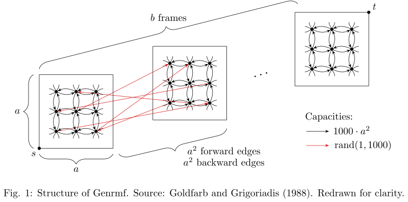
This graph was created by Goldfarb and Grigoriadis (1988) [1]. It consists of $$$b$$$ frames. Each frame is an $$$a \times a$$$ grid. Within each frame, neighboring vertices are connected in both directions by an edge of capacity $$$1000 \cdot a^2$$$. Between consecutive frames $$$f_i$$$ and $$$f_{i+1}$$$, there are $$$a^2$$$ forward edges from the vertices of $$$f_i$$$ to a random permutation of the vertices of $$$f_{i+1}$$$. Additionally there are $$$a^2$$$ backward edges from $$$f_{i+1}$$$ to a different random permutation of $$$f_i$$$. The capacities of these in-between edges are chosen uniformly at random from the range $$$[1, 1000]$$$.

AK

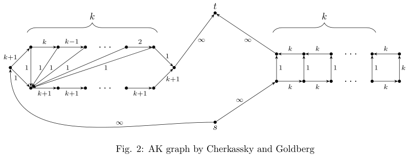
This graph was created by Cherkassky and Goldberg (1997) [2]. The following figure should describe the graph well.

About Benchmarking

For testing, I always set the maximum number of edges twice as high as the maximum number of vertices. Since Genrmf and AK have slightly different ratios ($$$m \approx 6n$$$ for Genrmf and $$$m \approx \frac{3}{2} n$$$ for AK), I will give them an unfair advantage: They only have to meet one of the bounds, either the vertex bound or the edge bound. So, for example, for $$$n \leq 1000$$$ and $$$m \leq 2000$$$, Genrmf is allowed to generate a graph with $$$n \approx 1000$$$ and $$$m \approx 6000$$$ and AK is allowed to generate a graph with $$$n \approx 1333$$$ and $$$m \approx 2000$$$. All other graphs must always satisfy both the vertex and the edge bounds.

The maximum edge capacity is always chosen as $$$10^9$$$.

For all graphs or algorithms where randomization is involved, the reported running times are averages over $$$10$$$ runs (on $$$10$$$ different random graphs).

Ford-Fulkerson with DFS

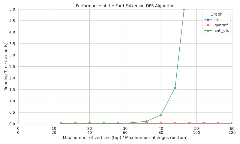
Implementing the Ford-Fulkerson algorithm using depth-first search to find augmenting paths is probably the simplest approach to solving the maximum flow algorithm. To be honest, I do not know graphs on which this algorithm requires $$$\Omega(m^2 \cdot U)$$$ time. However, on the following graphs, the running time is exponential, which should be bad enough. The graphs were created by Dean, Goemans and Immorlica (2006) [3].

I assume that the DFS prioritizes vertices with smaller indices. If instead it prioritizes edges based on their order in the input, the same behavior can be achieved by sorting the input edges lexicographically.

Randomized DFS

Ok, DFS with a predictable fixed order of the vertices can be exploited. But maybe randomly shuffling the adjacency lists before the start of the algorithm helps? Not really. You can still enforce the same behavior with high probability. Assume you have a vertex $$$a$$$ with two neighbors $$$b$$$ and $$$c$$$ and you want the randomized DFS to prioritize $$$b$$$ over $$$c$$$. Then you can replace $$$a$$$ with a path of vertices, all of which have an outgoing edge to $$$b$$$ and only the last one has an outgoing edge to $$$c$$$. The probability that $$$b$$$ is prioritized over $$$c$$$ will be $$$1 - 2^{-k}$$$, where $$$k$$$ is the length of the path.

Using this technique, we can recursively define bad graphs $$$G_{i,k}$$$ as seen in the figure below. The probability that the randomized DFS requires $$$2^i$$$ augmenting paths to compute the maximum flow on $$$G_{i,k}$$$ is $$$(1 - 2^{-k})^{4i}$$$.

Shortest Augmenting Paths (Edmonds-Karp, Dinic)

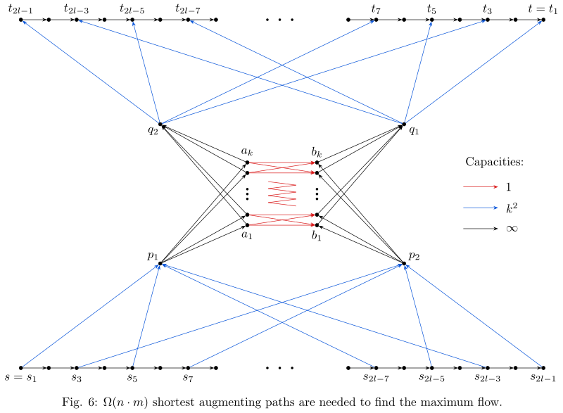
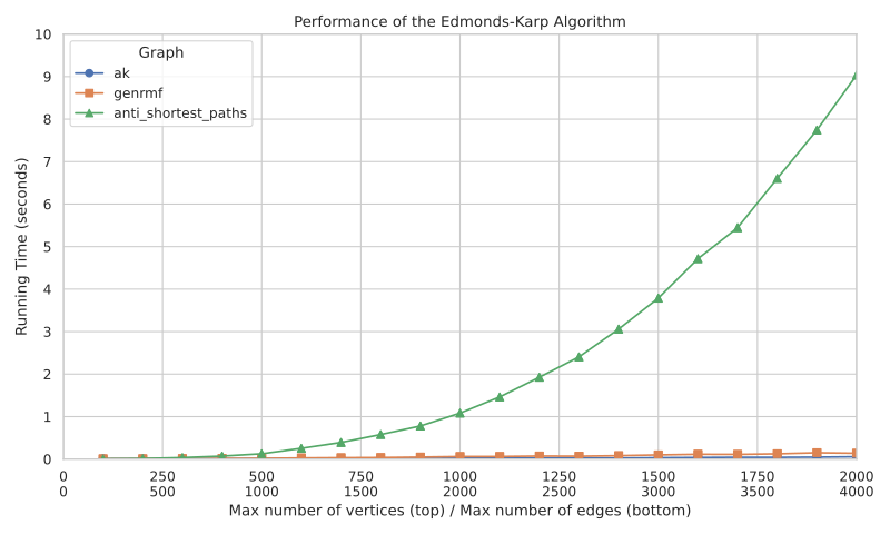
A worst-case graph for Edmonds-Karp and Dinic must require $$$\Omega(n \cdot m)$$$ shortest augmenting paths. The following graph is based on the graph by Zadeh (1972) [4].

Initially the shortest augmenting path is of the form

$$$s_1\rightarrow p_1\rightarrow a_i\rightarrow b_j\rightarrow q_1\rightarrow t_1.$$$

There are $$$k^2$$$ such paths, each with a residual capacity of one. After all these paths are found, the edges $$$(s_1,p_1)$$$, $$$(q_1,t_1)$$$ and all edges $$$(a_i,b_j)$$$ are saturated. Meaning they are reversed in the residual graph. Therefore the next $$$k^2$$$ shortest augmenting paths will be of the form

$$$s_1\rightarrow s_2\rightarrow s_3\rightarrow p_2 \rightarrow b_j\rightarrow a_i\rightarrow q_2\rightarrow t_3 \rightarrow t_2\rightarrow t_1.$$$

This repeats $$$l$$$ times. In total the number of augmenting paths is $$$l\cdot k^2$$$. So by choosing $$$k = \Theta(\sqrt{m})$$$ and $$$l = \Theta(n)$$$, we obtain a graph with $$$\mathcal{O}(n)$$$ vertices, $$$\mathcal{O}(m)$$$ edges and the required number of shortest augmenting paths is $$$\Omega(n \cdot m)$$$.

DFS with Scaling

This algorithm initializes a threshold $$$\Delta$$$ as a large power of two, for example $$$\Delta = 2^{\lfloor\log(U)\rfloor}$$$. It then finds augmenting paths with a DFS by only considering edges with residual capacity of at least $$$\Delta$$$. When no more such path exists, you divide $$$\Delta$$$ by two, and continue. When $$$\Delta = 1$$$ and no more augmenting paths exist, the maximum flow has been found. You can prove, that this strategy requires at most $$$\mathcal{O}(m \cdot \log(U))$$$ augmenting paths.

To achieve $$$\Omega(m \cdot \log(U))$$$ augmenting paths, we start with a complete bipartite graph containing $$$w^2$$$ edges, each of capacity $$$2^p-1$$$. The first threshold for which a path through the bipartite graph exists, is $$$\Delta = 2^{p-1}$$$. We want to have $$$w^2$$$ of those paths and we want that each of them has a capacity of exactly $$$2^{p-1}$$$. Therefore we add a copy of the Anti-DFS graph, which I described earlier. In this Anti-DFS graph, we increase all capacities by $$$2^{p-1}$$$ and make it large enough such that at least $$$w^2$$$ augmenting paths can be sent through it. Similarly we add Anti-DFS graphs for all thresholds $$$2^{p-2}, \dots, 2^0$$$.

In total, the DFS with Scaling algorithm requires $$$\Omega(w^2 \cdot p)$$$ augmenting paths, to find the maximum flow in this graph. So by setting $$$w = \Theta(\sqrt{m})$$$ and $$$p = \Theta(\log U)$$$ we achieve $$$\Omega(m \cdot \log(U))$$$ augmenting paths.

Additional Constraints

Dinic with Scaling

This is the same algorithm, as DFS with Scaling, only that the paths are found with Dinic (i.e., shortest paths) instead of depth-first search. Therefore the worst-case graph is also the same, only with Anti-Shortest-Paths-Graphs chained together instead of Anti-DFS graphs.

Additional Constraints

Most Improving Augmenting Paths

The Most Improving Augmenting Paths algorithm always chooses augmenting paths with the largest residual capacity. Similar to the capacity scaling algorithm, this strategy requires at most $$$\mathcal{O}(m \cdot \log(U))$$$ augmenting paths. The following graph was created by Queyranne (1980) [5].

First consider this graph with $$$10$$$ vertices and $$$17$$$ edges:

The most improving augmenting paths algorithm will find the following six augmenting paths:

Iteration	Path	Residual Capacity
1	$$$s \rightarrow a \rightarrow f \rightarrow g \rightarrow b \rightarrow h \rightarrow c \rightarrow d \rightarrow t$$$	8
2	$$$s \rightarrow f \rightarrow a \rightarrow g \rightarrow b \rightarrow c \rightarrow h \rightarrow t$$$	5
3	$$$s \rightarrow e \rightarrow f \rightarrow a \rightarrow b \rightarrow g \rightarrow h \rightarrow c \rightarrow t$$$	3
4	$$$s \rightarrow a \rightarrow f \rightarrow g \rightarrow b \rightarrow h \rightarrow c \rightarrow d \rightarrow t$$$	2
5	$$$s \rightarrow f \rightarrow a \rightarrow g \rightarrow b \rightarrow c \rightarrow h \rightarrow t$$$	1
6	$$$s \rightarrow e \rightarrow f \rightarrow a \rightarrow b \rightarrow g \rightarrow h \rightarrow c \rightarrow t$$$	1

You may notice a pattern. The residual path capacities are decreasing Fibonacci numbers. And the first three paths repeat themselves. In fact this pattern can be continued arbitrarily often just by increasing the edge capacities. Choosing the capacities as follows will cause $$$3k$$$ most improving augmenting paths.

Edges	Capacity
$$$sa, fg, bh, cd, dt$$$	$$$\sum_{i=1}^{k} F_{3i}$$$
$$$sf, ag, bc, ht$$$	$$$\sum_{i=1}^{k} F_{3i-1}$$$
$$$se, ef, ab, gh, ct$$$	$$$\sum_{i=1}^{k} F_{3i-2}$$$
$$$af, hc$$$	$$$F_{3k}$$$
$$$gb$$$	$$$F_{3k+1}$$$

Here $$$F_i$$$ are the Fibonacci numbers (i.e., $$$F_0 = 0$$$, $$$F_1 = 1$$$ and $$$F_i = F_{i-2} + F_{i-1}$$$ for $$$i \geq 2$$$). Since the Fibonacci numbers grow exponentially, the number of augmenting paths will be $$$\Omega(\log{U})$$$. In theory, to achieve $$$\Omega(m \cdot \log{U})$$$ augmenting paths, we could replace each edge with $$$\Omega(m)$$$ parallel edges. Or we could replace each vertex with a group of $$$\Omega(\sqrt{m})$$$ vertices and add complete bipartite graphs between the groups, instead of the original edges. However both these methods do not work in practice when the most improving paths are found with Dijkstra. Therefore in practice, the best graph, that I know of, achieves $$$\Omega(n \cdot \log{U})$$$ augmenting paths, by using $$$\Omega(n)$$$ copies of the above graph.

First-In-First-Out Preflow Push (FIFOPP)

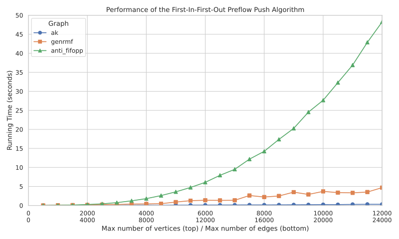
The following graph is inspired by the work of Cheriyan and Maheshwari (1989) [6]. I will only describe the general behavior of FIFOPP on the graph, and the behavior in practice is somewhat more complex. Please note that for the graph to work, the priority of the edges matters.

First, consider the following graph:

Initially a large flow excess is pushed into $$$p$$$. All this flow will then be pushed into $$$a_1$$$ and a single flow unit will be pushed to $$$b_1$$$, then to $$$q$$$ and then through the path of length $$$k$$$ toward $$$t$$$. The big flow excess that remained in $$$a_1$$$ is meanwhile pushed back to $$$p$$$ and then into $$$a_2$$$. Now another unit of flow is sent toward $$$t$$$. Overall $$$k$$$ units of flow are pushed toward $$$t$$$, so the total number of pushes is $$$\Omega(k^2) = \Omega(n^2)$$$.

To achieve a running time of $$$\Omega(n^3)$$$ we will reuse this structure $$$\Omega(n)$$$ times. To do that, we increase the length of the path and add edges from $$$q$$$ to every eighth vertex on the path. Each of capacity $$$k$$$. We do the same for vertex $$$p$$$, only the target vertices on the path are offset by four. And finally we set the capacity the edge $$$a_kb_k$$$ to infinity. The large flow excess will go back and forth between $$$p$$$ and $$$q$$$, a total of $$$k$$$ times. Each time it tries to go from $$$p$$$ to $$$q$$$ it will send $$$k$$$ unit flows toward $$$t$$$. The total required time is therefore $$$\Omega(k^3) = \Omega(n^3)$$$. (It is important, that the algorithm prioritizes $$$a_1 \dots a_{k-1}$$$ over $$$a_k$$$ and $$$b_1 \dots b_{k-1}$$$ over $$$b_k$$$).

Highest-Label Preflow Push (HLPP)

Again, the following graph is inspired by the work of Cheriyan and Maheshwari (1989) [6]. Again, I will only describe the general behavior of HLPP on the graph, and the behavior in practice is somewhat more complex. And again, please note that for the graph to work, the priority of the edges matters.

First consider the following gadget:

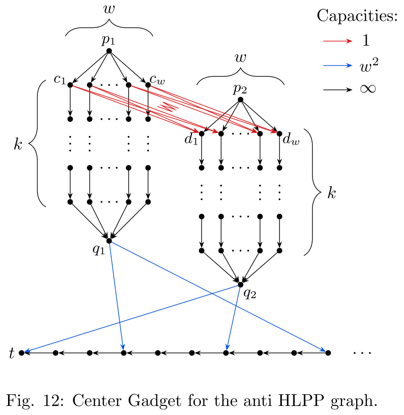
Assume a flow excess of value $$$w$$$ enters $$$p_1$$$. It will be pushed into $$$c_1$$$ and is then split up into $$$w$$$ flows of value $$$1$$$, which are pushed into the vertices $$$d_1, \dots, d_w$$$. Now they are pushed through $$$q_2$$$ toward $$$t$$$, causing a total of $$$w \cdot k$$$ pushes. This can repeat $$$w$$$ times, once for each $$$c_1, \dots, c_w$$$. After that, the edge $$$(q_2, t)$$$ and all edges $$$(c_i, d_j)$$$ are saturated.

Now assume a flow excess of value $$$w$$$ enters $$$p_2$$$. The shortest path to push it toward $$$t$$$ will be through $$$d_1$$$ and then to split up into $$$w$$$ flows of value $$$1$$$ into the vertices $$$c_1, \dots, c_w$$$ and then through $$$q_1$$$ toward $$$t$$$. Of course, the HLPP algorithm will not immediately realize that this is the shortest path. But after pushing the flow back and forth between $$$p_2$$$ and $$$q_2$$$ a few times, it will at some point push everything into $$$c_1, \dots, c_w$$$ and behave as described. (Here it is important that the algorithm prioritizes edges that lead away from $$$t$$$, i.e., pointing upward in the figure). So in total there are again $$$k \cdot w$$$ pushes. And again this can be repeated $$$w$$$ times, once for each $$$d_1, \dots, d_w$$$.

After that, there can again be a sequence of $$$w$$$ pushes of value $$$w$$$ into $$$p_1$$$, and then again a sequence of $$$w$$$ pushes of value $$$w$$$ into $$$p_2$$$. And so on.

We will choose $$$w = \Theta(\sqrt{m})$$$ and $$$k = \Theta(n / \sqrt{m})$$$. Therefore, if we are able to send $$$\Omega(n)$$$ sequences of $$$w$$$ pushes, each of value $$$w$$$, into $$$p_1$$$ and $$$p_2$$$ (alternating between them), then this will result in a total of $$$\Omega(n \cdot w \cdot w \cdot k) = \Omega(n^2 \cdot \sqrt{m})$$$ pushes.

To achieve these $$$\Omega(n)$$$ sequences of $$$w$$$ pushes into $$$p_1$$$ and $$$p_2$$$, we start by adding the following side gadgets:

The source will push an excess of value $$$w^2$$$ into $$$a_1$$$. Which will then be split into $$$w$$$ pushes of value $$$w$$$ through the side gadget into $$$b_1$$$. There it will realize it is in a dead end and the algorithm will one by one push each of these $$$w$$$ flow excesses back through $$$a_1$$$ and then into $$$p_1$$$ exactly as we wanted. After this process, the side gadget is empty again and could be reused.

Ideally we want to have more than one source vertex. Initially one source vertex should send a flow of $$$w^2$$$ into $$$a_1$$$. Then after all this flow has been processed, a second source should get activated that sends a flow of $$$w^2$$$ into $$$a_2$$$. This should repeat $$$\Omega(n)$$$ times, alternating between pushing flow into $$$a_1$$$ and into $$$a_2$$$.

We can actually simulate this behavior of having multiple sources. The real source $$$s$$$ will be connected to $$$2l$$$ vertices which serve as the auxiliary sources. We add an edge from these auxiliary sources directly to $$$t$$$. This has the effect that their height label is $$$1$$$. Meaning they will always have the lowest label (i.e., the lowest priority to be chosen by HLPP). So HLPP will only activate a new auxiliary vertex once all flow from the previous source has been fully processed. See the figure below for the final Anti-HLPP graph. By choosing $$$l = \Theta(n)$$$, $$$k = \Theta(n / \sqrt{m})$$$ and $$$w = \Theta(\sqrt{m})$$$, we obtain a graph with $$$\mathcal{O}(n)$$$ vertices and $$$\mathcal{O}(m)$$$ edges. And HLPP requires at least $$$2l \cdot w \cdot w \cdot k = \Omega(n^2 \cdot \sqrt{m})$$$ pushes.

Reasons why the performance on the Anti-HLPP graph is not worse than on Genrmf:

Genrmf has the property that more flow is sent deep into the graph, than can ultimately be pushed into $$$t$$$. To push this flow back to $$$s$$$ the algorithm must relabel a lot of vertices $$$\Omega(n)$$$ times. This results in a running time of $$$\Omega(n \cdot m)$$$.
Remember that I allowed Genrmf to use about $$$3$$$ times more edges than Anti-HLPP.
The constant factor of Anti-HLPP is very low (about $$$\frac{1}{150}$$$).

And the graph sizes are not large enough, such that $$$\frac{1}{150} n^2 \cdot \sqrt{m}$$$ beats $$$3 \cdot n \cdot m$$$.

HLPP with Global Relabeling and Gap Heuristics

The Global Relabeling heuristic and the Gap heuristic do not help on the Anti-HLPP graph. However, they help a lot on Genrmf.

Comparing all Algorithms

Of course, all these graphs represent only asymptotic worst-case scenarios. It is quite likely that other worst-case graphs exist with much higher constant factors.

Thanks for reading. If you know about any other bad maximum flow graphs, I would love to know about them :)

References

\documentclass[tikz]{standalone} \usepackage{tikz} \usetikzlibrary{arrows.meta} \definecolor{MyRed}{rgb}{0.9, 0.4, 0.4} \definecolor{MyBlue}{rgb}{0.35, 0.55, 0.9} \begin{document} \begin{tikzpicture}[x=1.0mm, y=1.0mm] \tikzstyle{vertex} = [circle, draw=black, fill=black, scale=0.3] \tikzstyle{unit_edge} = [-{Stealth[scale=0.8]},MyRed!150] \tikzstyle{inf_edge} = [-{Stealth[scale=0.8]}] \tikzstyle{kk_edge} = [-{Stealth[scale=0.8]},MyBlue!150] \node[vertex] at (0, 0) (s01) {}; \node[vertex] at (8, 0) (s02) {}; \node[vertex] at (16, 0) (s03) {}; \node[vertex] at (24, 0) (s04) {}; \node[vertex] at (32, 0) (s05) {}; \node[vertex] at (40, 0) (s06) {}; \node[vertex] at (48, 0) (s07) {}; \node[vertex] at (56, 0) (s08) {}; \node[vertex] at (94, 0) (s09) {}; \node[vertex] at (102, 0) (s10) {}; \node[vertex] at (110, 0) (s11) {}; \node[vertex] at (118, 0) (s12) {}; \node[vertex] at (126, 0) (s13) {}; \node[vertex] at (134, 0) (s14) {}; \node[vertex] at (142, 0) (s15) {}; \node[vertex] at (150, 0) (s16) {}; \node[vertex] at (0, 100) (t01) {}; \node[vertex] at (8, 100) (t02) {}; \node[vertex] at (16, 100) (t03) {}; \node[vertex] at (24, 100) (t04) {}; \node[vertex] at (32, 100) (t05) {}; \node[vertex] at (40, 100) (t06) {}; \node[vertex] at (48, 100) (t07) {}; \node[vertex] at (56, 100) (t08) {}; \node[vertex] at (94, 100) (t09) {}; \node[vertex] at (102, 100) (t10) {}; \node[vertex] at (110, 100) (t11) {}; \node[vertex] at (118, 100) (t12) {}; \node[vertex] at (126, 100) (t13) {}; \node[vertex] at (134, 100) (t14) {}; \node[vertex] at (142, 100) (t15) {}; \node[vertex] at (150, 100) (t16) {}; \node[vertex] at (40, 30) (p1) {}; \node[vertex] at (110, 30) (p2) {}; \node[vertex] at (110, 70) (q1) {}; \node[vertex] at (40, 70) (q2) {}; \node[vertex] at (65, 41) (a1) {}; \node[vertex] at (65, 44) (a2) {}; \node[vertex] at (65, 56) (a3) {}; \node[vertex] at (65, 59) (a4) {}; \node[vertex] at (85, 41) (b1) {}; \node[vertex] at (85, 44) (b2) {}; \node[vertex] at (85, 56) (b3) {}; \node[vertex] at (85, 59) (b4) {}; \draw[inf_edge] (s01) -- (s02); \draw[inf_edge] (s02) -- (s03); \draw[inf_edge] (s03) -- (s04); \draw[inf_edge] (s04) -- (s05); \draw[inf_edge] (s05) -- (s06); \draw[inf_edge] (s06) -- (s07); \draw[inf_edge] (s07) -- (s08); \draw[inf_edge] (s09) -- (s10); \draw[inf_edge] (s10) -- (s11); \draw[inf_edge] (s11) -- (s12); \draw[inf_edge] (s12) -- (s13); \draw[inf_edge] (s13) -- (s14); \draw[inf_edge] (s14) -- (s15); \draw[inf_edge] (s15) -- (s16); \draw[inf_edge] (t01) -- (t02); \draw[inf_edge] (t02) -- (t03); \draw[inf_edge] (t03) -- (t04); \draw[inf_edge] (t04) -- (t05); \draw[inf_edge] (t05) -- (t06); \draw[inf_edge] (t06) -- (t07); \draw[inf_edge] (t07) -- (t08); \draw[inf_edge] (t09) -- (t10); \draw[inf_edge] (t10) -- (t11); \draw[inf_edge] (t11) -- (t12); \draw[inf_edge] (t12) -- (t13); \draw[inf_edge] (t13) -- (t14); \draw[inf_edge] (t14) -- (t15); \draw[inf_edge] (t15) -- (t16); \draw[kk_edge] (s01) -- (p1); \draw[kk_edge] (s03) -- (p2); \draw[kk_edge] (s05) -- (p1); \draw[kk_edge] (s07) -- (p2); \draw[kk_edge] (s10) -- (p1); \draw[kk_edge] (s12) -- (p2); \draw[kk_edge] (s14) -- (p1); \draw[kk_edge] (s16) -- (p2); \draw[kk_edge] (q2) -- (t01); \draw[kk_edge] (q1) -- (t03); \draw[kk_edge] (q2) -- (t05); \draw[kk_edge] (q1) -- (t07); \draw[kk_edge] (q2) -- (t10); \draw[kk_edge] (q1) -- (t12); \draw[kk_edge] (q2) -- (t14); \draw[kk_edge] (q1) -- (t16); \draw[inf_edge] (p1) -- (a1); \draw[inf_edge] (p1) -- (a2); \draw[inf_edge] (p1) -- (a3); \draw[inf_edge] (p1) -- (a4); \draw[inf_edge] (p2) -- (b1); \draw[inf_edge] (p2) -- (b2); \draw[inf_edge] (p2) -- (b3); \draw[inf_edge] (p2) -- (b4); \draw[inf_edge] (a1) -- (q2); \draw[inf_edge] (a2) -- (q2); \draw[inf_edge] (a3) -- (q2); \draw[inf_edge] (a4) -- (q2); \draw[inf_edge] (b1) -- (q1); \draw[inf_edge] (b2) -- (q1); \draw[inf_edge] (b3) -- (q1); \draw[inf_edge] (b4) -- (q1); \draw[unit_edge] (a1) -- (b1); \draw[unit_edge] (a1) -- (b2); \draw[unit_edge] (a2) -- (b1); \draw[unit_edge] (a2) -- (b2); \draw[unit_edge] (a3) -- (b3); \draw[unit_edge] (a3) -- (b4); \draw[unit_edge] (a4) -- (b3); \draw[unit_edge] (a4) -- (b4); \draw node at (75, 0) {\Huge\dots}; \draw node at (75, 100) {\Huge\dots}; \draw node at (65, 51) {\Huge\vdots}; \draw node at (85, 51) {\Huge\vdots}; \draw node at (0, -3) {$$$s = s_1$$$}; \draw node at (16, -3) {$$$s_3$$$}; \draw node at (32, -3) {$$$s_5$$$}; \draw node at (48, -3) {$$$s_7$$$}; \draw node at (102, -3) {$$$s_{2l-7}$$$}; \draw node at (118, -3) {$$$s_{2l-5}$$$}; \draw node at (134, -3) {$$$s_{2l-3}$$$}; \draw node at (150, -3) {$$$s_{2l-1}$$$}; \draw node at (150, 103) {$$$t = t_1$$$}; \draw node at (134, 103) {$$$t_3$$$}; \draw node at (118, 103) {$$$t_5$$$}; \draw node at (102, 103) {$$$t_7$$$}; \draw node at (48, 103) {$$$t_{2l-7}$$$}; \draw node at (32, 103) {$$$t_{2l-5}$$$}; \draw node at (16, 103) {$$$t_{2l-3}$$$}; \draw node at (0, 103) {$$$t_{2l-1}$$$}; \draw node at (38, 32) {$$$p_1$$$}; \draw node at (113, 32) {$$$p_2$$$}; \draw node at (113, 68) {$$$q_1$$$}; \draw node at (38, 68) {$$$q_2$$$}; \draw node at (65, 38) {$$$a_1$$$}; \draw node at (65, 62) {$$$a_k$$$}; \draw node at (85, 38) {$$$b_1$$$}; \draw node at (85, 62) {$$$b_k$$$}; \draw[-,MyRed!150] (79,46.5) -- (71,47.5) -- (79,48.5) -- (71,49.5) -- (79,50.5) -- (71,51.5) -- (79,52.5) -- (71,53.5); \draw node at (136, 59) {Capacities:}; \draw[unit_edge] (127, 52) -- (137, 52); \draw node at (140, 52) {$$$1$$$}; \draw[kk_edge] (127, 46) -- (137, 46); \draw node at (141, 46) {$$$k^2$$$}; \draw[inf_edge] (127, 40) -- (137, 40); \draw node at (141, 40) {$$$\infty$$$}; \draw node at (75, -10) {Fig. 6: $$$\Omega(n\cdot m)$$$ shortest augmenting paths are needed to find the maximum flow.}; \end{tikzpicture} \end{document}

Комментарии (21)

Написать комментарий?

NNEDAA

14 месяцев назад, скрыть # |

+79

💀

→ Ответить

segtreebeats

orz

Abhinav_2004

← Rev. 2 →

-21

This blog offers an insightful and rigorous exploration of worst-case graphs for various maximum flow algorithms, highlighting the deep gap between theoretical complexity and practical performance.

Thanks for posting

Pov: My mind is not working after reading this blog .

jeroenodb

+11

Ford-Fulkerson using DFS, does one DFS search from the source, and then it increases the flow by at least $$$1$$$, or it terminates. Shouldn't its complexity be $$$O((n+m)U)$$$?

Um_nik

14 месяцев назад, скрыть # ^ |

+19

$$$U$$$ is the limit on one edge capacity, maxflow is (theoretically) $$$mU$$$.

Oops yes. That upperbound seems indeed hard to achieve. You kinda need multiedges for it. But maybe it's almost achievable with the construction in the blog. This conatruction uses $$$O(\log(U))$$$ edges. But by using multiedges we can build more levels on top of this construction (using $$$2^k$$$ parallel, weight $$$U$$$ edges). We can build $$$\log_2(m) - O(1)$$$ levels more. This means the construction can send $$$O(m U)$$$ units of flow one at a time, and then each time at the top level you take at least $$$O(m)$$$ looping through all the multiedges.

lotusblume

← Rev. 4 →

+21

Wow, I have never realized that this extension results in $$$\Omega(mU)$$$ paths. Then the construction does actually achieve the worst case.

It is not true $$$\Omega(mU)$$$, but rather $$$\Omega$$$(min($$$mU, 2^{m/4}$$$)). So we can not get arbitrarily many paths for a fixed $$$m$$$ by just increasing $$$U$$$.

But getting arbitrarily many paths for DFS, by just increasing $$$U$$$ is impossible. Because you can proof that the DFS algorithm will never find the same path twice. (In that sense DFS is even superior to Most-Improving-Augmenting-Paths).

Proof

We define a total order on $$$s-t$$$ paths: to compare two paths $$$P$$$ and $$$P'$$$, look at the first vertex where their chosen outgoing edges differ, let them be $$$e$$$ and $$$e'$$$ and compare those two edges by their priority in the algorithm. We say $$$e \lt e'$$$ (and consequently $$$P \lt P'$$$) if $$$e$$$ is prioritized over $$$e'$$$.

To proof that no augmenting path appears twice, we show that whole sequence of augmenting paths is strictly increasing.

Let $$$G$$$ be the residual graph before an augmentation, and $$$P=e_1,\dots,e_k$$$ the augmenting path found by the DFS in $$$G$$$. Let $$$G'$$$ be the residual graph after augmenting along $$$P$$$, and let $$$P'=e'_1,\dots,e'_\ell$$$ be the next augmenting path found by the DFS in $$$G'$$$.

First, $$$P'\neq P$$$: along $$$P$$$, at least one forward residual edge becomes saturated (the bottleneck), so that edge is not available in $$$G'$$$, and the identical path cannot reappear immediately.

Let $$$i$$$ be the first index where $$$P$$$ and $$$P'$$$ differ. Then $$$e_j=e'_j$$$ for all $$$j \lt i$$$, and both paths are at the same vertex $$$u$$$ just before choosing their $$$i$$$-th edge. Let $$$e_i=(u,v)$$$ and $$$e'_i=(u,v')$$$. We will show $$$e_i \lt e'_i$$$, and consequently $$$P \lt P'$$$.

Assume for contradiction that $$$e_i \gt e'_i$$$.

Claim 1. The edge $$$e'_i = (u,v')$$$ is already present as a residual edge in $$$G$$$.

Proof of Claim 1. The only residual edges whose status changes from $$$G$$$ to $$$G'$$$ are edges on $$$P$$$ (their forward residual capacity decreases) and their reverses (their reverse residual capacity increases). Thus an edge that was absent in $$$G$$$ but present in $$$G'$$$ must be the reverse of an edge used by $$$P$$$ in the forward direction. If $$$(u,v')$$$ were such a newly created edge, then $$$(v',u)$$$ would lie on $$$P$$$. But $$$P$$$ and $$$P'$$$ share the same prefix up to $$$u$$$, so $$$u$$$ is visited before $$$v'$$$ on $$$P$$$. And since augmenting paths are simple, $$$P$$$ cannot later traverse $$$(v',u)$$$ (that would revisit $$$u$$$). Contradiction. Therefore $$$(u,v')$$$ is already in $$$G$$$.

Let $$$S$$$ be the set of vertices on the prefix of $$$P$$$ from $$$s$$$ up to and including $$$u$$$. Consider the graph $$$G-S$$$ obtained from $$$G$$$ by deleting $$$S$$$. Let $$$W$$$ be the set of vertices reachable from $$$v'$$$ in $$$G-S$$$.

Claim 2. $$$t\notin W$$$.

Proof of Claim 2. When the DFS at $$$u$$$ in $$$G$$$ chooses the next edge, it tries outgoing edges in the fixed order. Since $$$e'_i=(u,v')$$$ is prioritized over $$$e_i=(u,v)$$$ by assumption, if $$$t$$$ were reachable from $$$v'$$$ in $$$G-S$$$, the DFS would have followed $$$(u,v')$$$ and eventually reached $$$t$$$, producing an augmenting path that used $$$(u,v')$$$ instead of $$$(u,v)$$$. That contradicts the choice of $$$P$$$.

Now look at $$$G'$$$ and the path $$$P'$$$. Because $$$P'$$$ is simple and shares the prefix ending at $$$u$$$ with $$$P$$$, the suffix of $$$P'$$$ starting from $$$v'$$$ does not visit any vertex of $$$S$$$. Hence, in $$$G'-S$$$, there is a path from $$$v'$$$ to $$$t$$$. Consequently, in $$$G'-S$$$ there must be at least one edge leaving $$$W$$$ (otherwise $$$t$$$ would still be unreachable from $$$v'$$$ because $$$v' \in W$$$).

But in $$$G-S$$$, by definition of $$$W$$$, there are no residual edges leaving $$$W$$$. Therefore some edge leaving $$$W$$$ is newly present in $$$G'-S$$$ that was not present in $$$G-S$$$.

The only way such a new leaving edge can appear when passing from $$$G$$$ to $$$G'$$$ is as the reverse of an edge of $$$P$$$ that goes into $$$W$$$. However, $$$P$$$ cannot enter $$$W$$$: if $$$P$$$ ever reached a vertex of $$$W$$$ in $$$G-S$$$, then it would be impossible for $$$P$$$ to continue to $$$t$$$. Therefore $$$P$$$ does not touch $$$W$$$, and no new edge leaving $$$W$$$ can be created. Contradiction.

Therefore our assumption was false, and $$$e_i = (u,v)$$$ must be prioritized over $$$e'_i = (u,v')$$$, that is $$$e_i \lt e'_i$$$. Consequently $$$P$$$ < $$$P'$$$. By induction, the whole sequence of augmenting paths is strictly increasing. In particular, no augmenting path can appear twice.

+145

This is amazing. Thank you very much.

The graphs could be more informative, though. Log scale, or if you want to show that the complexity is a specific function, you can make the ordinate scale as that function, so the points will be on a line.

+39

Thank you a lot for the suggestion. I tried it for Dinic and HLPP.

Dinic

HLPP

It is really nice to see the straight lines :)

tiom4eg

+18

Illustrations in your blog look incredible! You made them in LaTeX or with some other tool (I'm talking about graph structure ones, of course)?

And blog in general is very good, thank you for your hard work!

Thank you, I am glad you liked it.

Yes, I created the graphs with LaTeX, TikZ. Here is for example the code for the Anti-Shortest-Paths graph:

anti_shortest_paths.tex

Edit: It seems like all '$' are displayed as '$$$'. But they should all be single '$'.

arthur_9548

Thank you very much, lotusblume. This is really an amazing blog! Very nice study and great descriptions.

As a problemsetter, this will be very useful for me as a reference when preparing flow problems in the future :)

We need more flow problems in codeforces contests :D

+13

I agree!

izanbf

11 месяцев назад, скрыть # |

Amazing work!

enze_qwq

If I don't remember it wrong, I believe there is one approach using LCT + dinic and it could potentially get to $$$O(nmlogn)$$$.

Spheniscine

11 месяцев назад, скрыть # ^ |

I've been told that using LCTs introduces quite a high constant factor, and thus isn't particularly useful for the purposes of competitive programming. Hadn't tried it myself though.