Monogon's blog

By Monogon, history, 9 months ago, In English

To whom it may concern,

Today I was reading some recent problems when I stumbled upon this div2B. 1956B - Nene and the Card Game. At first, it seems like an innocent game theory problem, until I read the following sentence.

Nene is very smart so she always selects cards optimally in order to maximize her score in the end of the game (after $$$2n$$$ rounds). If she has several optimal moves, she selects the move that minimizes your score in the end of the game.

This struck me as a bit odd, because in most game theory problems on Codeforces, it's a win/lose/draw game, or the player wants to maximize the difference between their score and their opponent's score, or they want to maximize their own score and all outcomes have the same sum of scores for the two opponents (which is equivalent). But Nene's objective is most peculiar, where she doesn't care about how many points her opponent has at all, until she cannot get any more for herself and then it is the only thing she cares about.

Now, what does the problem say is the strategy of Nene's opponent (you)?

...what is the maximum number of points you can get by taking your turns optimally?

Hmm, it seems that you do not care about Nene's score, although she cares about your score. Oh well.

At this moment I thought, "is this problem even well-defined?" What does an optimal strategy mean in this game? We seem to take it for granted that it even makes sense to talk about an "optimal strategy" at all. There are a few possible concepts of what an optimal strategy could mean. Maybe it means playing the move that gives you the best guaranteed score, assuming the worst case for your opponent's decisions. Or maybe it means playing the move that gives you the best outcome assuming that your opponent is rational and plays optimally. Yet another interpretation could involve Alice and Bob agreeing to collaborate, if they see a path that makes them both better-off than if they competed.

In most game theory problems on Codeforces, we are dealing with a two-player, zero-sum (or constant-sum), turn-based, finite, perfect-information game. In these cases, multiple interpretations of optimal play turn out to be equivalent. The one where you try to optimize your guaranteed score is called Maximin and the one where you try to optimize your score assuming a rational opponent is called Minimax. Both of these solution concepts are equivalent for this class of games.

However the idea of "maximize your score first, then minimize your opponent's score second" seems to imply that we are outside of zero-sum territory (otherwise maximizing your own score would be enough). We cannot guarantee that Minimax = Maximin in non-zero-sum games. For example, consider this simple example game.

Alice goes first.
Choice 1: Alice and Bob both get 1 point, game ends.
Choice 2: Go to Bob

If Bob has a turn:
Choice 1: Alice gets 0 points, Bob gets 1 point, game ends.
Choice 2: Alice gets 2 points, Bob gets 2 points, game ends.
  • Maximin: Suppose Alice wants to maximize her guaranteed score, assuming the worst case. Then she should make choice 1, because she can guarantee 1 point, while the worst case in choice 2 is 0 points.
  • Minimax: Suppose Alice wants to maximize her score assuming that Bob is rational and will try to maximize his own score. Then she should go with choice 2, since Bob will rationally get 2 points for each of them, which is better than 1 point.

In this example, we see how non-zero-sum games can result in different optimal strategies depending on which convention we choose. In general, the problem statement would need to be clear about which convention we are using.

So, what about this div2B problem? Is it well-defined? Technically, yes it is. After analyzing the mechanics of the game, you will notice that the sum of scores of the two players is the same in all outcomes. In fact, for each type of card, one of them will be played first and the other will be played second, resulting in $$$1$$$ point for one of the players. So the sum of scores will always be $$$n$$$ in every outcome, meaning it's a constant-sum game in disguise.

So, what lesson can we take from my incoherent rambling? Mainly, optimal play in game theory is surprisingly nuanced. In my opinion, problems on Codeforces should be immediately clear that they are well-defined, and this div2B problem requires a key observation in order to realize that it is well-defined. Maybe when we have zero-sum games in the future, we should make it clear that it is zero-sum, even if it's just a statement like "We can prove that the sum of the players' scores is the same in all outcomes", and maybe linking to a resource about the definition of optimal play in zero-sum games.

Full text and comments »

  • Vote: I like it
  • +176
  • Vote: I do not like it

By Monogon, history, 14 months ago, In English

Source: https://en.m.wikipedia.org/wiki/International_Collegiate_Programming_Contest

The 2011 ACM-ICPC World Finals were held in Orlando, Florida and hosted by main sponsor IBM. The contest was initially scheduled to be held in Sharm el-Sheikh, Egypt in February, but was moved due to the political instability associated with the Arab Spring

Rescheduling of World Finals 22&23

Full text and comments »

  • Vote: I like it
  • +142
  • Vote: I do not like it

By Monogon, 2 years ago, In English

Good morning!

In this blog, I will present an online algorithm that can perform priority-queue-like undoing on a data structure, given a few assumptions. I will also present and solve a generalization of that problem.

For context, I highly recommend reading this blog that shows how to solve the easier problem of queue-like undoing. That blog gave me the inspiration for the trick I will describe here, but I will still try to write this blog so that it can be understood without it. Thank you Noam527 for introducing such a great trick to the competitive programming community.

[Tutorial] Supporting Queue-like Undoing on DS

Acknowledgment

Huge thanks go to peltorator for hosting a blog contest. His generous prize of $300 got many people to write blogs on new, interesting ideas, and it was one of the main reasons I wrote this blog. I'm honored to win the prize, so thanks again to peltorator!

Problem Statement

Let $$$D$$$ be a data structure that supports updates and queries. We require $$$D$$$ to be commutative, meaning that if we apply a set of updates and then a query, the answer to the query will be the same regardless of the order that we applied the updates. Let's assume that if we apply a sequence of $$$n$$$ updates to $$$D$$$, then each update will take $$$O(T(n))$$$ non-amortized time. Let's also assume that we have a way to undo the most recent update in $$$O(T(n))$$$ time (this can usually be supported by maintaining a stack of changes we've made to the internal state of $$$D$$$, and undoing the changes on the top of the stack).

Now, we would like to the solve the problem of supporting the following types of operations online:

  1. Apply an update to $$$D$$$ with an associated priority $$$p$$$. (Assume all priorities are unique).
  2. Undo the update in $$$D$$$ that has the highest priority. (Recall that the updates are commutative).
  3. Answer a query about $$$D$$$.

Given a sequence of $$$n$$$ updates and queries, we will solve this problem in $$$O(n T(n) \log n)$$$ time. In other words, each operation takes $$$O(T(n)\log n)$$$ amortized time.

Subproblems

There are a few special cases of the above problem that we get for free.

First, if the priorities are inserted in decreasing order, this is the same as the queue-like undoing problem described in Noam's blog.

Second, if we remove the online requirement, then we can support arbitrary deletions in the same time complexity. This is because we can pre-compute priorities that reduces the problem to the one described above. We simply say that the priority of an update is inversely correlated to its deletion time. This subproblem of offline deletion can also be solved using a different well-known trick.

Idea

The idea is that we have a stack $$$S$$$ of updates in the order that we applied them to $$$D$$$. If the highest priority update coincides with the top of the stack, that's great, we can just pop it and undo the most recent update to $$$D$$$. However if we need to undo an update that's buried deep within the stack, we need to spend a lot of work undoing all of the updates that come after it, and then pushing them back onto the stack.

Fortunately, we have some flexibility that can help us save time. Firstly, we can decide to push the updates back onto the stack in a different order than they were before. This can help us because we can choose to put higher priority updates closer to the top of the stack, which saves us time later on. Secondly, we can choose to pop even more elements than required for the current undo operation. It can sometimes help to dig deeper into the stack because it can make up for the work we've already done. For example, suppose we've already popped a lot of elements to get the highest priority update. If the second highest priority update is close behind it, it might be worth popping it out as well so that it will be more accessible later.

Solution

In this solution, the operations of applying new updates and answering queries will be handled in a straightforward manner. When we apply an update we push it directly to the stack and apply it to $$$D$$$. When we answer a query, we don't touch the stack at all.

Then when we need to undo the highest priority update, we need to decide the number of updates to pop from the stack. Let's choose the smallest number $$$k\ge 1$$$ such that the following condition holds: The $$$\lceil\frac{k}{2}\rceil$$$ highest priority updates in the stack are among the top $$$k$$$ positions of the stack.

After we pop these $$$k$$$ updates, we push them back onto the stack in such a way that the $$$\lceil\frac{k}{2}\rceil$$$ highest priority updates are all on top of the stack, sorted in increasing order.

Details

Now, it's a bit of a non-trivial detail to efficiently check if the desired condition has been met. The proof of complexity will rely on the fact that processing $$$k$$$ updates on the stack takes $$$O(\log n + k T(n))$$$ time. To make the result as general as possible, we want to support the case where $$$T(n)=1$$$, so our overhead costs should be $$$O(\log n + k)$$$. This means we can't afford to do something such as sorting the top $$$k$$$ elements by priority.

In order to satisfy this requirement, let's say that in addition to the stack of updates we also maintain a set data structure of the updates, ordered by priority. (Such as std::set in C++). When we add an update, it takes $$$O(\log n)$$$ time to insert into the set, and when we pop an update, it takes $$$O(\log n)$$$ time to delete it from the set. In the undo operation, as we iterate $$$k$$$ in increasing order, we simultaneously iterate through the $$$\lceil\frac{k}{2}\rceil$$$ elements of the set with the highest priority. Let's say that the stack-depth of an update is the number of updates currently above it on the stack. As we iterate through the set, we keep track of the largest stack-depth of those elements, and compare with $$$k$$$. If $$$k$$$ is larger than the largest stack-depth, the condition is met. Otherwise, we need to continue iterating $$$k$$$.

After we decide to stop iterating, we can efficiently push all the elements back onto the stack. First we can push all the elements that are not among the highest $$$\lceil \frac{k}{2}\rceil$$$ priorities. We can push them in the same order that they originally appeared on the stack, for example. (Remember we can't afford to sort them.) Then, we push the remaining elements in increasing order of priority. That can be done efficiently by iterating through the top elements of the set, and doesn't require us to sort from scratch.

And so, we can see that processing $$$k$$$ elements of the stack can be done in $$$O(\log n + k T(n))$$$ time, which is good enough for the proof of time complexity of the entire algorithm.

Complexity Analysis

Let's say that the cost of an operation is the number of stack elements processed. So, a push operation has a cost of $$$1$$$ and an undo operation has a cost of $$$k$$$, where $$$k$$$ is the number of elements of the stack popped in that operation. We will ignore query operations. If $$$C_i$$$ is the cost of the $$$i$$$-th operation, then we will show that $$$\sum_{i=1}^n C_i = O(n\log n)$$$. Note that this is sufficient to show that the overall time complexity is

$$$\sum_{i=1}^n (\log n + C_i T(n)) = n\log n + T(n) \sum_{i=1}^n C_i = O(n T(n)\log n).$$$

Now we will show that for any two indices $$$i<j$$$, we have $$$2(j-i)\ge \min(C_i, C_j).$$$ This is clearly true if either operation $$$i$$$ or $$$j$$$ is a push operation, so let's assume that they are both undo operations. Assume for contradiction that the inequality does not hold, and let $$$i$$$, $$$j$$$ be a counterexample where $$$j-i$$$ is the smallest possible.

Let $$$k=\min(C_i,C_j)$$$. Since $$$k\le C_i$$$, we know that after operation $$$i$$$, the $$$\lceil \frac{k}{2}\rceil$$$ highest priority updates are on top of the stack in increasing order. Let $$$U$$$ be the set of those updates. Suppose that between operations $$$i$$$ and $$$j$$$ there are $$$m_1$$$ push operations and $$$m_2$$$ pop operations. So, there are at most $$$m_1$$$ new elements and at least $$$\lceil\frac{k}{2}\rceil-m_2$$$ elements remaining from $$$U$$$ at the time before operation $$$j$$$.

Since $$$C_j\ge k$$$, we know that either it stopped before it passed over all the remaining elements of $$$U$$$ when processing the stack, or the condition was not satisfied the first time it encountered all the remaining elements of $$$U$$$. In the first case, there needed to be at least $$$\lceil\frac{k}{2}\rceil$$$ additions between $$$i$$$ and $$$j$$$, so $$$j-i\ge \lceil\frac{k}{2}\rceil$$$ which contradicts our assumption. In the second case, this means that $$$\lceil\frac{k}{2}\rceil-m_2<m_1$$$, otherwise the condition would have been satisfied. But then we have that

$$$j-i>m_1+m_2>\left\lceil\frac{k}{2}\right\rceil \ge \frac12 \min(C_i, C_j)$$$

contradicting our assumption. Therefore, the inequality always holds.

Let $$$y_c$$$ be the number of operations $$$i$$$ such that $$$C_i\ge c$$$. The above fact shows that more expensive operations are farther apart, so we know that $$$y_c\le 1+\frac{2n}{c}$$$. Finally, we have that

$$$\sum_{i=1}^n C_i = \sum_{c=1}^n y_c\le \sum_{c=1}^n (1+\frac{2n}{c}) = n + 2n \sum_{c=1}^n \frac1c = O(n\log n).$$$

Generalization to Multiple Priorities

Although priority-queue-like undoing is pretty cool, I realized it's still not general enough to support deque-like undoing, where we can undo either the oldest update or the most recent update. More generally, what if priorities are $$$d$$$-dimensional vectors, and we want to undo the update that has the largest priority in a specified dimension? That is, we would like to support the following operations:

  1. Apply an update with associated priority vector $$$(p_1,\ldots, p_d)$$$.
  2. Undo the update whose priority vector has the largest value in dimension $$$i$$$.

Note that this can simulate deque-like undoing because we can use priorities $$$(p, -p)$$$.

Solution

We can support this generalization in the following way. At the end of an undo operation, push elements to the stack in a cyclic manner. For example if there are three dimensions $$$x$$$, $$$y$$$, $$$z$$$, then we make sure the element with the largest $$$x$$$ value is on top, then of the remaining elements make sure the element with the largest $$$y$$$ value is on top, then $$$z$$$, then $$$x$$$, and so on.

When we pop elements, we stop when the following condition is met: For each dimension $$$i=1\ldots d$$$, the $$$\lceil \alpha k\rceil$$$ elements with the highest priorities in dimension $$$i$$$ are among the top $$$k$$$ positions of the stack. Here, $$$\alpha$$$ is some constant between $$$0$$$ and $$$\frac1d$$$ will be decided later. For the implementation detail, we can maintain $$$d$$$ different set data structures, with the $$$i$$$-th one sorting the updates according to the $$$i$$$-th dimension.

Complexity Analysis

The complexity analysis is very similar; all we have to show is that there is some value $$$\beta$$$ such that for any two operations $$$i<j$$$, we have $$$\beta(j-i)\ge \min(C_i, C_j)$$$. Then we can guarantee that the complexity is $$$O(\beta n T(n) \log n)$$$.

Suppose that $$$C_i\ge k$$$. Then for each dimension, the largest $$$\alpha k$$$ elements of that dimension are present among the top $$$d\alpha k$$$ positions of the stack after operation $$$i$$$. Let $$$U$$$ be the set of those $$$d\alpha k$$$ elements. Let's say we apply $$$m_1$$$ additions and $$$m_2$$$ deletions between $$$i$$$ and $$$j$$$.

Since $$$C_j\ge k$$$, we know that either it stopped before it passed over all the remaining elements of $$$U$$$ when processing the stack, or the condition was not satisfied the first time it encountered all the remaining elements of $$$U$$$. In the first case, there needed to be at least $$$(1-d\alpha)k$$$ additions between $$$i$$$ and $$$j$$$, so $$$(j-i)\ge (1-d\alpha)k$$$.

In the second case, assume without loss of generality that the condition failed on the first dimension when it first encountered the remaining elements of $$$U$$$. There are at least $$$\alpha k-m_2$$$ remaining elements from $$$U$$$ with the highest priorities in dimension $$$1$$$ and at most $$$d\alpha k + m_1-m_2$$$ overall elements at the time the condition fails. Therefore,

$$$\alpha k - m_2<\alpha(d\alpha k + m_1-m_2).$$$

Let $$$m=m_1+m_2$$$ and $$$\lambda=\frac{m_1}{m}$$$ be the proportion of additions out of the operations. If we replace $$$m_1=\lambda m$$$ and $$$m_2=(1-\lambda)m$$$ and rearrange, we get

$$$\frac{m}{k} > \frac{\alpha - d\alpha^2}{\alpha \lambda + (1-\alpha) (1-\lambda)}.$$$

Let's define a function $$$f(\alpha, \lambda)$$$ to be the right-hand side of that inequality. The worst case is when $$$f(\alpha, \lambda)$$$ is small because it gives us the weakest lower bound for $$$m$$$. Note that the denominator is a convex combination of $$$\alpha$$$ and $$$(1-\alpha)$$$. So depending on which is larger, the worst case is either $$$\lambda=0$$$ or $$$\lambda=1$$$. Therefore, if we set

$$$\beta=\frac{1}{\min(1-d\alpha, f(\alpha, 0), f(\alpha, 1))},$$$

then the above claim holds.

This means that if we treat $$$d$$$ as a constant, the complexity is $$$O(nT(n)\log n)$$$.

Optimizing $$$\alpha$$$

The complexity analysis above is somewhat incomplete, because we haven't seen how to choose an optimal $$$\alpha$$$ value or how the complexity scales up with $$$d$$$. To get the best guarantee of complexity, we want $$$\beta$$$ to be as small as possible, or $$$\frac{1}{\beta}=\min(1-d\alpha, f(\alpha, 0), f(\alpha, 1))$$$ to be as large as possible.

First, consider the case where $$$d=1$$$. In this case, $$$f(\alpha, 0)=\alpha$$$ and $$$f(\alpha, 1)=1-\alpha$$$. We can easily see that the optimal value of $$$\min(\alpha, 1-\alpha)$$$ happens at $$$\alpha_{opt}=\frac12$$$.

Now let's consider $$$d\ge 2$$$. We have that $$$\alpha<\frac1d\le\frac12\le 1-\frac1d<1-\alpha$$$ which means that $$$f(\alpha, 0)\le f(\alpha, 1)$$$. It's also always true that $$$f(\alpha, 0)\le 1-d\alpha$$$. So, we really just need to maximize $$$f(\alpha, 0)$$$ over $$$0<\alpha<\frac1d$$$.

With some calculus, we find that the optimal value is

$$$\alpha_{opt}=1-\sqrt{1-\frac1d}.$$$

Also with the help of my friend Mr. Wolfram Alpha, we find that

$$$\lim_{d\to\infty}\frac{1}{d\ f(\alpha_{opt}, 0)}=4.$$$

This means that

Unable to parse markup [type=CF_MATHJAX]

and so our final complexity becomes $$$O(dnT(n)\log n)$$$.

As a mini-disclaimer, I'll note that the optimized $$$\alpha$$$ values are only theoretical and a different value might be better in a practical implementation. With that out of the way, here is a reference table of approximate values for a few dimensions. It would be interesting to see how they compare on a benchmark implementation.

$$$d$$$ $$$\alpha_{opt}$$$ $$$\beta$$$
$$$1$$$ $$$0.5$$$ $$$2$$$
$$$2$$$ $$$0.292893$$$ $$$5.828427$$$
$$$3$$$ $$$0.183503$$$ $$$9.898979$$$
$$$4$$$ $$$0.133975$$$ $$$13.928203$$$
$$$5$$$ $$$0.105573$$$ $$$17.944272$$$

Thanks for coming to my TED talk.

Full text and comments »

  • Vote: I like it
  • +409
  • Vote: I do not like it

By Monogon, history, 3 years ago, In English

The first Codeforces contest I authored included this problem: 1345B - Card Constructions.

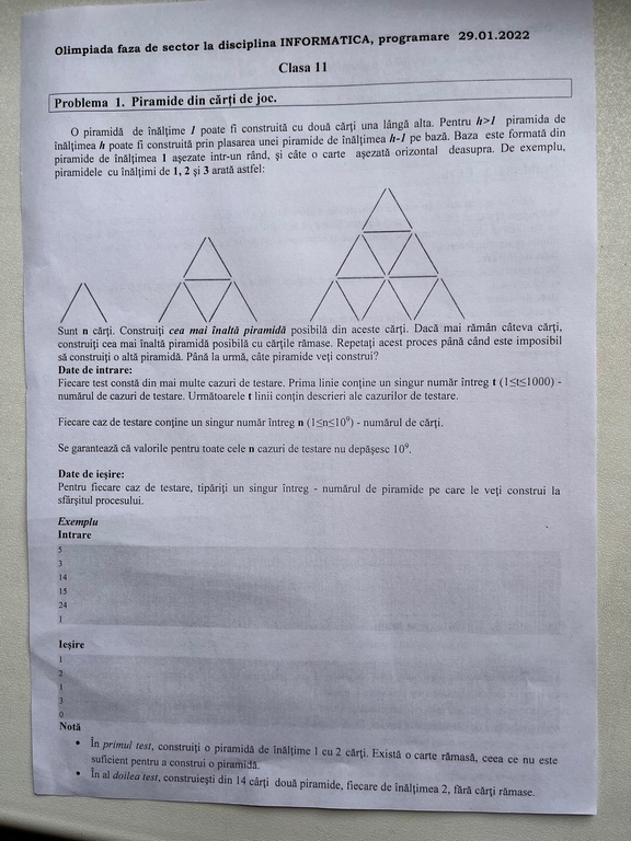
Almost 2 years later, the following problem appeared in the Moldovan first state regional of OI:

Now, maybe it's just a notorious coincidence, like when a problem someone authors on Codeforces happened to appear on Topcoder before. In those cases, at least there are noticeable differences in presentation. But the author of this OI problem seems to have magically written the statement in the same way, designed the same picture, came up with the same constraints, and created the same sample test case.

Several questions come to mind. Can contestants have an unfair advantage if some have seen this problem before? Is someone being paid to invent problems for OI and steals an online problem instead? When a problem is used on Codeforces, who owns the intellectual property rights to it? Of all problems I created why didn't they steal a better one?

That's all I have for today, and don't forget to smash that like button.

Full text and comments »

  • Vote: I like it
  • +700
  • Vote: I do not like it

By Monogon, history, 3 years ago, In English

There are a lot of programming problems where a collection of intervals comes up, either directly or indirectly. In this tutorial, I want to present a nice way to visualize a collection of intervals, and how you can solve problems with it.

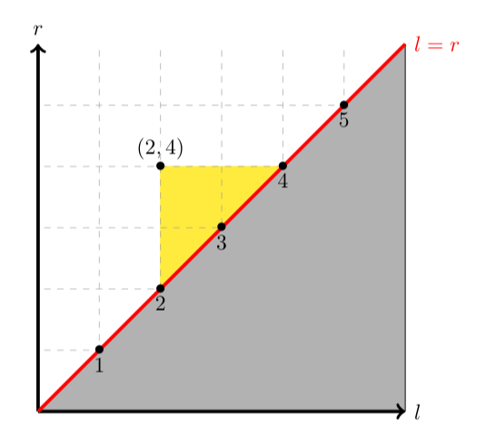
An interval $$$[l, r]$$$ is just a pair of integers $$$l$$$ and $$$r$$$ such that $$$l\le r$$$. Let's make a 2D plot where the horizontal axis is $$$l$$$ and the vertical axis is $$$r$$$. Then our interval will be represented by the 2D point $$$(l, r)$$$. But an interval is more than just a pair of numbers: it describes the set of points $$$x$$$ such that $$$l\le x\le r$$$.

How can we visually tell whether a number $$$x$$$ is covered by an interval? Well, we can represent it by a point $$$(x, x)$$$ in the plane. Then we can imagine that the interval's 2D point can see down and right, and the interval covers all the points it can see.

Here's an example where we see how the interval $$$[2, 4]$$$ covers the points $$$2$$$, $$$3$$$, and $$$4$$$.

Great, we have a visualization for how an interval covers points. But we also want to talk about how intervals relate to each other. For example, intervals can be nested, or they can be disjoint, or something else.

Let's classify the $$$6$$$ possible ways two intervals can relate to each other.

  1. An interval $$$[l_1, r_1]$$$ covers an interval $$$[l_2, r_2]$$$ if $$$l_1\le l_2\le r_2\le r_1$$$.

  2. An interval $$$[l_1, r_1]$$$ is covered by an interval $$$[l_2, r_2]$$$ if $$$l_2\le l_1\le r_1\le r_2$$$.

  3. An interval $$$[l_1, r_1]$$$ is strictly left of an interval $$$[l_2,r_2]$$$ if $$$l_1\le r_1 < l_2\le r_2$$$.

  4. An interval $$$[l_1, r_1]$$$ is strictly right of an interval $$$[l_2, r_2]$$$ if $$$l_2\le r_2 < l_1\le r_1$$$.

  5. An interval $$$[l_1, r_1]$$$ intersects left of an interval $$$[l_2,r_2]$$$ if $$$l_1\le l_2\le r_1\le r_2$$$.

  6. An interval $$$[l_1, r_1]$$$ intersects right of an interval $$$[l_2, r_2]$$$ if $$$l_2\le l_1\le r_2\le r_1$$$.

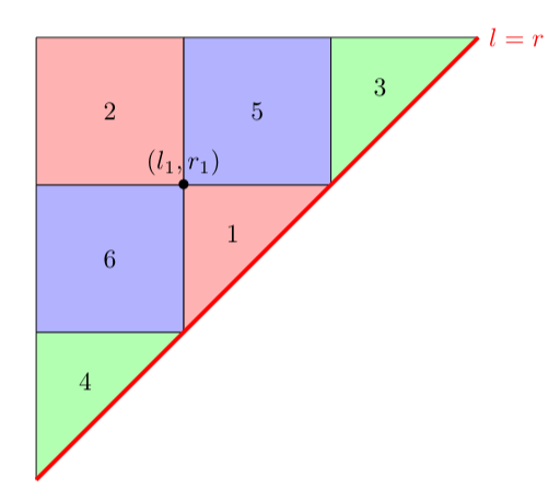
Note that there is some symmetry. For example, if one interval covers another interval, then the second interval is covered by the first interval. So, relations $$$1$$$ and $$$2$$$ are opposites, relations $$$3$$$ and $$$4$$$ are opposites, and relations $$$5$$$ and $$$6$$$ are opposites. Now, if we fix an interval $$$(l_1, r_1)$$$ we can make $$$6$$$ different regions in the plane: one for each relation. I colored opposite relations the same color.

Next, we're going to look at some example problems.

Problem 1. Nested Ranges Check

https://cses.fi/problemset/task/2168

Given $$$n$$$ ranges, your task is to determine for each range if it contains some other range and if some other range contains it.

There are two parts to this problem, so let's focus on one part for now. For each interval $$$(l, r)$$$, we want to check if it's covered by another interval. In other words, we want to check if its region $$$2$$$ is nonempty.

For an interval to be in region $$$2$$$, it must be left and up from it. Let's process all intervals in increasing order of $$$l$$$, so that the "left of" condition just becomes "previously processed". So, we just need to ask for each interval, if there exists a previously processed interval above it.

If any previously processed interval is above $$$(l, r)$$$, then definitely the one with maximum $$$r$$$ will be above it. So we don't need to check all the previous intervals by brute force: just remember the maximum $$$r$$$ value seen so far and remember it.

There's one small issue we skipped over: when we sorted all intervals by $$$l$$$, we didn't say what to do in the case of ties. In other words, if two intervals have the same $$$l$$$ value, should we process the lower or higher one first? Well, if there are two intervals with the same $$$l$$$ value, then the larger one is considered to cover the second. This means the interval with smaller $$$r$$$ should definitely be processed after the one with larger $$$r$$$. So in the case of ties for $$$l$$$ value, we should process them in decreasing order of $$$r$$$.

Now we've solved one of the two parts. For the other part, we want to check for each interval, if it covers another interval. We can actually use the exact same idea, except we will sort decreasing by $$$l$$$, break ties in increasing order of $$$r$$$, and remember the minimum $$$r$$$ value of all processed intervals.

The total complexity will be $$$O(n\log n)$$$ from sorting.

Problem 2. Nested Ranges Count

https://cses.fi/problemset/task/2169

Given $$$n$$$ ranges, your task is to count for each range how many other ranges it contains and how many other ranges contain it.

This is very similar to the previous problem, but this time we want to count ranges instead of just checking. Just like last time, let's start with only focusing on counting for each interval, how many other intervals contain it. Also like last time, let's process all intervals in increasing order of $$$l$$$, and break ties with decreasing order of $$$r$$$.

Now when we process an interval $$$(l, r)$$$, we need to count how many previously processed intervals are above it. We should maintain some kind of data structure of the processed intervals, where we can insert a value and query how many are above a certain value.

If we do coordinate compression, we can make all the intervals have values between $$$1$$$ and $$$2n$$$ without changing any of the relationships between them. Now we can store the processed $$$r$$$ values in a Fenwick tree, for example. To insert a new $$$r$$$ value, we update the Fenwick tree to increment position $$$r$$$. To answer how many values are above $$$r$$$, we query the range $$$[r, 2n]$$$.

Again, the other half of this problem is the same except for the sorting order and we want to count the number of $$$r$$$ values below instead of above.

The total complexity will be $$$O(n\log n)$$$, due to sorting and answering queries.

Problem 3. Largest Nested Interval Subset

Given $$$n$$$ intervals, find the size of the largest possible subset of intervals with the following property: for any pair of intervals, one contains the other.

First, we can describe the "nested subset" property in a nicer way: If the intervals are sorted decreasing by length $$$r-l$$$, then the first interval contains the second interval, and the second interval contains the third interval, and so on. Geometrically, this means we're looking for a path of points that moves only down and right. Now we can see that this is basically the same as the longest decreasing subsequence problem.

We can solve this problem in a similar way as before: sort all intervals in increasing order of $$$l$$$ and break ties with decreasing order of $$$r$$$. This time, we're going to use dynamic programming. For an interval $$$[l_i, r_i]$$$ we'll compute $$$dp_i$$$, which we define to be the largest nested subset of intervals such that $$$[l_i, r_i]$$$ is the smallest interval. The final answer will be the maximum $$$dp_i$$$ value.

To compute $$$dp_i$$$, we have the formula

$$$dp_i=1+\max\limits_{j:r_i\le r_j}(dp_j),$$$

where we assume $$$j$$$ is only allowed to be a previously processed interval. If there exist no valid $$$j$$$ then we set $$$dp_i=1$$$. Just like the Nested Ranges Count problem, we can maintain a data structure that can support point updates (to insert a new $$$dp_i$$$ value) and range max queries (to find the maximum $$$dp_j$$$ value corresponding to $$$r_j\ge r_i$$$). For example, a segment tree that supports range maximum queries will work here.

The total complexity will be $$$O(n\log n)$$$ due to sorting and segment tree queries.

Problem 4. Interesting Sections

1609F - Interesting Sections

There is an array of non-negative integers $$$a_1,a_2,\ldots, a_n$$$. Count the number of segments $$$[l, r]$$$ such that: 1. The minimum and maximum numbers are found on the segment of the array starting at l and ending at r. 2. the binary representation of the minimum and maximum numbers have the same number of bits equal to 1.

First, for each index, we want to know the largest interval on which it's the minimum element, and the largest interval on which it's the maximum element. We can precompute all these intervals in linear time with a monotonic stack idea, for example. Let's say the interval where $$$a_i$$$ the minimum element is $$$[l_1(i),r_1(i)]$$$ and the interval where it's the maximum element is $$$[l_2(i),r_2(i)]$$$. If there's a tie for the minimum (maximum) element in a range, we always pick the first occurrence to be the minimum (maximum).

Now, for each index $$$i$$$, let's consider the set of intervals $$$[l,r]$$$ on which $$$a_i$$$ is the minimum element. We simply require it to contain index $$$i$$$, and for it to be contained in $$$[l_1(i), r_1(i)]$$$. In the plane, this is just a rectangle: $$$l_1(i)\le l\le i$$$ and $$$i\le r\le r_1(i).$$$ Similarly, we have a rectangle for the maximum case.

Let's say that a rectangle is red if it came from the minimum case, and blue if it came from the maximum case. First, notice that no two rectangles of the same color intersect because a range has a unique minimum and maximum by our tie-breaking rule. Our task is to calculate how many lattice points are the intersection of a red and blue rectangle, and both of them have the same "group number", namely the popcount of their corresponding $$$a_i$$$ values.

Let's just offset rectangles according to their group number so that rectangles of different group numbers definitely don't intersect, and rectangles of the same group are offset by the same amount.

The only thing we need to compute is the area of intersection of red rectangles and blue rectangles. We can find the area of intersection of these rectangles in $$$O(n\log n)$$$ time with a sweepline and segment tree. The rectangle union problem is similar, which can be found on CSES: https://cses.fi/problemset/task/1741

For the rectangle intersection problem, we need our segment tree to maintain two things: 1. maximum value on a range, and 2. number of occurrences of the maximum element. It needs to support range increment/decrement updates and range queries. When the sweepline enters a rectangle, we increment its range, and when it exits a rectangle, we decrement its range. A value $$$2$$$ in the segment tree means there are both red and blue rectangles covering it, so the number of occurrences of $$$2$$$ describes how much intersection there is between red and blue at the sweepline's current position.

Full text and comments »

  • Vote: I like it
  • +255
  • Vote: I do not like it

By Monogon, history, 3 years ago, In English

I hope you enjoyed the contest!

1615A - Closing The Gap

Author: PurpleCrayon

Tutorial

1615B - And It's Non-Zero

Author: PurpleCrayon

Tutorial

1615C - Menorah

Author: Monogon

Tutorial

1615D - X(or)-mas Tree

Author: PurpleCrayon

Tutorial

1615E - Purple Crayon

Author: PurpleCrayon

Tutorial

1615F - LEGOndary Grandmaster

Author: PurpleCrayon

Tutorial

1615G - Maximum Adjacent Pairs

Author: BledDest

Tutorial

1615H - Reindeer Games

Author: Monogon

Tutorial

Full text and comments »

  • Vote: I like it
  • +178
  • Vote: I do not like it

By Monogon, history, 3 years ago, In English

In this tutorial I'll introduce potentials as it applies to directed graphs and discuss a few of its applications. I haven't seen many resources about this topic, so I decided to write one.

Prerequisites:

  • Shortest path algorithms (Dijkstra and Bellman-Ford)
  • For the Min Cost Max Flow section, you should be familiar with Ford-Fulkerson. But you can benefit from this blog with just the Johnson's Algorithm section if you're not familiar with flows.

Introduction

For notation, let's say there is a weighted, directed graph $$$G=(V,E)$$$. Let $$$n=|V|$$$ and $$$m=|E|$$$. For simplicity, let's assume there are no loops or multiple edges between the same pair of nodes in the same direction. For an edge $$$u\to v$$$, we will use $$$w(u\to v)$$$ to denote its weight.

Let's motivate the idea of a potential, so the definition doesn't seem to come out of nowhere. In shortest paths, you may be aware that negative edges create a lot of issues. First, it's possible that negative cycles exist. In that case, it's possible for a path to have arbitrarily small weight, and we say that $$$\mathrm{dist}(u\to v)=-\infty$$$. (By the way, we allow a path to revisit vertices. If we required a simple path, then it's NP-complete.)

Even if there are no negative cycles, the negative edges are still problematic for us. Dijkstra's algorithm can give incorrect results, and we typically use Bellman-Ford instead, which has a worse complexity. Dijkstra's is $$$O(m\log n)$$$ while Bellman-Ford is $$$O(mn)$$$. Technically, Dijkstra's algorithm can be improved to $$$O(m+n\log n)$$$ with Fibonacci heaps, but it's not very important for the purposes of this blog. I mention it anyway in case you're confused why other resources have a different complexity.

One possible idea to deal with negative edges is to "reweigh" the graph so that all weights are non-negative, and it still encodes the information of shortest paths in the original graph. Obviously, we can't just replace the weights with whatever we want. One way we can modify weights is to pick a vertex $$$v$$$, increase the weights of incoming edges to $$$v$$$ by some real value $$$x$$$, and decrease the weights of outgoing edges from $$$v$$$ by the same amount $$$x$$$. This way, any path that goes through $$$v$$$ will have the same weight as before. Therefore, the only affected paths are the ones that begin or end at $$$v$$$. But we can observe that any path beginning or ending in $$$v$$$ will just be offset by $$$x$$$, and a shortest path will remain the shortest.

Now, we have the motivation to define a potential. The idea is that we want to apply this kind of vertex offset for all vertices independently in such a way that all the new weights are non-negative.

Definition: A function $$$p:V\to \mathbb{R}$$$ is called a potential of graph $$$G$$$ if for every edge $$$(u\to v)\in E$$$, it holds that $$$w(u\to v)+p(u)-p(v)\ge 0$$$.

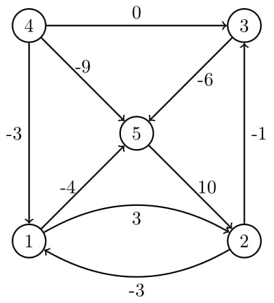
For an example, consider this graph:

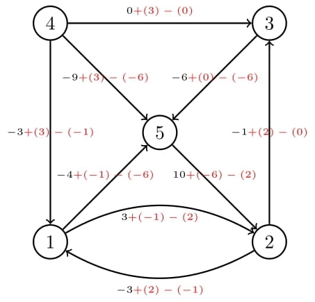
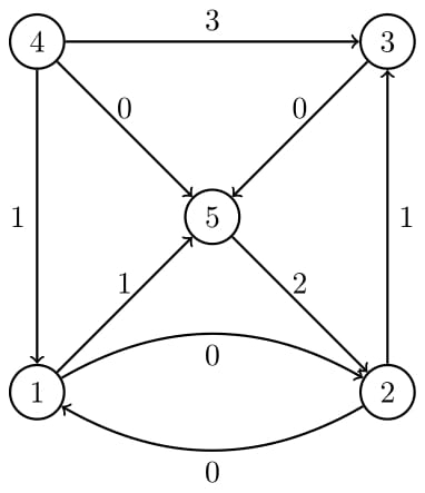
Let's apply the potential $$$p$$$, where $$$p(1)=-1,\ p(2)=2,\ p(3)=0,\ p(4)=3,\ p(5)=-6$$$, and confirm that the new edge weights are all non-negative.

Since the new edge weights are indeed all non-negative, $$$p$$$ is a valid potential. Now, let's confirm the fact that information of path weights is preserved. For example, take the path $$$4\to3\to 5\to 2\to 1$$$. In the original graph, it has weight $$$0-6+10-3=1$$$. In the new graph, it has weight $$$3+0+2+0=5$$$, and we expect it to be offset by the difference of the endpoints' potentials, $$$p(4)-p(1)=3-(-1)=4$$$, which is correct.

Note that if a graph has a negative cycle, then you cannot create a potential for it. This is because the weight of a cycle is unchanged by the reweighing.

Johnson's Algorithm

Given our graph $$$G$$$, we would like to compute length of the shortest path from $$$u$$$ to $$$v$$$, for all pairs $$$(u, v)$$$. For simplicity, let's assume there are no negative cycles in the graph. Perhaps the best algorithm you know about for this problem is Floyd-Warshall, which works in $$$O(n^3)$$$. (It works correctly for negative edges).

Johnson's Algorithm solves this problem more efficiently for sparse graphs, and it uses the following steps:

  1. Compute a potential $$$p$$$ for the graph $$$G$$$.
  2. Create a new weighting $$$w'$$$ of the graph, where $$$w'(u\to v)=w(u\to v)+p(u)-p(v)$$$.
  3. Compute all-pairs shortest paths $$$\mathrm{dist}'$$$ with the new weighting.
  4. Convert the distances back to the original graph, with the equation $$$\mathrm{dist}(u\to v)=\mathrm{dist}'(u\to v)-p(u)+p(v)$$$.

We need to go into more detail about how steps 1 and 3 can be done. Step 3 is easier to understand, so let's address it first. The weighting $$$w'$$$ is all non-negative, so we can use Dijkstra's algorithm to get correct distances. We simply run Dijkstra's algorithm once for every vertex $$$u$$$, to get the distances from $$$u$$$ to every other vertex. Since we run Dijkstra's algorithm $$$n$$$ times, and each time takes $$$m\log n$$$, the complexity for this stage is $$$O(nm\log n)$$$. Technically, it can be improved to $$$O(n(n\log n+m))=O(n^2\log n+nm)$$$ if you use Fibonacci heaps.

Now, how do we do step 1? The key idea is that shortest path values themselves satisfy the requirement of a potential! In fact, let's fix some vertex $$$s$$$, and assign $$$p(v)=\mathrm{dist}(s\to v)$$$ for all vertices $$$v$$$. Assume for contradiction that $$$p$$$ is not a potential. Then there is some edge $$$u\to v$$$ such that $$$w(u\to v)+p(u)-p(v)<0$$$. This means that $$$\mathrm{dist}(s\to v)>\mathrm{dist}(s\to u)+w(u\to v)$$$. This means that if we take the shortest path from $$$s$$$ to $$$u$$$, then take the edge from $$$u$$$ to $$$v$$$, the total weight will be smaller than the shortest distance from $$$s$$$ to $$$v$$$. Clearly, this is impossible, so $$$p$$$ is in fact a potential.

Actually, I lied to you. The above proof is only correct if the chosen vertex $$$s$$$ can reach all vertices $$$v$$$. Otherwise, we would have infinite potentials which is not allowed by the definition. But we're almost there. Let's simply create a brand new vertex $$$s$$$, and create an edge $$$s\to v$$$ with weight $$$0$$$ for every vertex $$$v$$$. We will define the potential based on the shortest distance from $$$s$$$, and it will be correct. Note that the property of a potential is still valid if we delete some vertices and edges, so it's not a problem to remove $$$s$$$ after we compute the potential. Also note that when we add $$$s$$$ and those extra edges, we do not create a negative cycle since no edges are incoming to $$$s$$$.

Now, you might be thinking, "wait, I thought the point of a potential is to help us compute shortest paths, and now you're telling me we need to use shortest paths to compute the potential? I want my upvote back!" But remember, we're trying to compute all-pairs shortest paths. Running an algorithm like Bellman-Ford from every starting vertex would be expensive. But here, we're only running such an algorithm once, from the new vertex $$$s$$$. Then we use a more efficient algorithm (Dijkstra) for the all-pairs part. So for this step 1, we just run Bellman-Ford once on the graph with the new vertex $$$s$$$. The complexity of step 1 is $$$O(nm)$$$.

Overall, step 3 is the bottleneck and Johnson's algorithm has complexity $$$O(nm\log n)$$$ (or $$$O(n^2\log n + nm)$$$ if you use Fibonacci heap).

Min Cost Max Flow

I will present the minimum cost maximum flow (MCMF) problem, show how to solve it, then show how potentials can make it faster. If you want formal proofs, I recommend resources below. My proofs here will be business casual.

We are given a directed graph $$$G=(V, E)$$$. There are two special nodes $$$s$$$ and $$$t$$$, called the source and sink. Every edge $$$u\to v$$$ has a capacity $$$c(u\to v)$$$ and a cost $$$w(u\to v)$$$. A flow is defined as an assignment $$$f:E\to \mathbb{R}$$$ such that:

  • For every edge $$$u\to v$$$, the flow sent along this edge is non-negative and does not exceed the capacity. Formally, $$$0\le f(u\to v)\le c(u\to v)$$$.
  • For every vertex $$$u$$$ ($$$u\ne s$$$, $$$u\ne t$$$), flow-out equals flow-in. Formally,
$$$\sum\limits_{v:(u\to v)\in E} f(u\to v) =\sum\limits_{v:(v\to u)\in E}f(v\to u)$$$

The value of a flow is defined as $$$\sum\limits_{u:(s\to u)\in E}f(s\to u)$$$. The cost of a flow is defined as $$$\sum\limits_{(u\to v)\in E}f(u\to v)w(u\to v)$$$.

The maximum flow problem simply asks to maximize the value of the flow. The MCMF problem asks us to find the minimum cost flow among all flows with the maximum possible value.

Let's recall how to solve the maximum flow problem with Ford-Fulkerson. We iteratively send flow from $$$s$$$ to $$$t$$$ by finding an augmenting path, which is a path of edges from $$$s$$$ to $$$t$$$ using only edges that are below full capacity. Also, we include reversed edges that allow us to send flow "back". We can find such a path with DFS.

In MCMF, we do almost the same thing, except that we must find the shortest path each iteration. A forward edge $$$u\to v$$$ has weight $$$w(u\to v)$$$ and the corresponding back edge has weight $$$-w(u\to v)$$$. We ignore edges at full capacity (and back edges whose corresponding forward edge has no flow to send back). Casually, we can understand that shortest paths will be correct by induction. If we have an optimal flow with value $$$k$$$, then consider the optimal flow with value $$$k+1$$$. The difference will include a path from $$$s$$$ to $$$t$$$ and some cycles. A cycle cannot cause a decrease in cost, otherwise we can find a better flow with value $$$k$$$. So it's optimal to just augment a path. In particular, an optimal augmenting path must be the shortest with our given weighting.

Since this graph has negative edges, we might use Bellman Ford each iteration. But with potentials, we can do better. We already know that if we're given a potential for the graph, then the shortest path can be computed easily with Dijkstra. But when we send flow along an augmenting path, it changes which edges are at full capacity, which can make the potential invalid for the next iteration.

How can we compute the potential for the next iteration more efficiently than running Bellman-Ford every time? It turns out that we can use the shortest path results from the Dijkstra to assign the potentials for the next iteration for free. This works because the shortest distances create a potential for the edges involved, as mentioned in the Johnson's algorithm section. So we just need to check that the edges that change from sending flow do not create an issue. Suppose an edge becomes full capacity. Then it is removed from our graph for shortest path computations, and it cannot make the potential invalid. Suppose an edge was at full capacity but not after sending flow along the augmenting path. In this case, the reversed edge satisfied the inequality before sending flow, which automatically means this edge satisfies it (since $$$w(u\to v)=-w(v\to u)$$$).

Now, given a potential for one iteration we can compute it for the next iteration for free. But what about the first iteration? In many cases, the costs are all non-negative and we can just use $$$p(u)=0$$$ for the potential. Otherwise if there are no negative cycles, we can run Bellman-Ford to get the initial potential. I'm not aware of how to deal with negative cost cycles, and I haven't yet seen it appear in a problem. If you're knowledgeable about negative cycles in MCMF, I'd love to hear about it in the comments.

Ignoring a possible Bellman-Ford or similar to compute the initial potential, the complexity is $$$O(F(m\log n))$$$. With Fibonacci heap, you get $$$O(F(m + n\log n))$$$. Note that for very dense graphs, it's optimal to do the simple $$$O(n^2)$$$ Dijkstra algorithm which doesn't use any heap.

Implementation, with initial potential of 0

Resources

Practice Problems

Full text and comments »

  • Vote: I like it
  • +387
  • Vote: I do not like it

By Monogon, history, 3 years ago, In English

First of all, Codeforces is great and I like its UI much better than other platforms. But there is one issue that annoys me repeatedly. I haven't seen it discussed in a blog yet (apologies if I missed it), so I thought I'd make this request.

Sometimes I revisit a problem I solved before, and I want to see my submission. Then I get confused because I don't see my submission in the lower right corner of the problem page. Eventually, I find that I need to view a different link that shows the same problem.

Now, it makes some sense that the same problem should have different links. For example, if I'm viewing the problem in a virtual contest, I want to see the correct short-name depending on the division. If the problem is div2C, I want to see C if I got there from div2, or A if from div1. Another example is that if a problem came from the contest, I don't want to see tags, but I might if I got there from the problemset.

So, a problem can have multiple links. For example, all these 6 links go to the same problem:

Yet, I can only see a submission I made on two of them. On top of these, there's the gym section where people can create even more links to the same problem.

I hope what I'm requesting isn't too hard to implement, since all different links to the same problem ultimately point back to the same Polygon problem ID. Specifically, it would be really cool if:

  • When viewing a problem, I can see the submissions I've made to it regardless of what link I used.
  • When viewing a problem, I can easily navigate to the other links that are the same problem.
  • When I submit a problem from the contest page as an author/coordinator, it will shine a green light on the problemset page that induces a well-earned dopamine hit. (Currently it seems to only work if I submit it from the problemset page, not the contest page).

Is there a good reason why one wouldn't want to view the past submissions or mark a problem with green for all versions? Should gym links be treated differently than the "official" links? Is this more challenging to implement than I estimated? Will I ever pass MikeMirzayanov in contribution? Is it rated? Please leave your opinion in the comments below.

Full text and comments »

  • Vote: I like it
  • +362
  • Vote: I do not like it

By Monogon, history, 3 years ago, In English
  • Vote: I like it
  • +734
  • Vote: I do not like it

By Monogon, history, 3 years ago, In English

North American ICPC participants were all ready to go to Orlando, Florida for a week-long event including NAPC (North America Programming Camp) and NAC (North America Championship), which will decide the 2021 World Finalists from North America. With less than a week's notice, and after all travel plans were arranged by the teams, the following announcement was made.

Dear NAC — NAPC Participant,

Due to the surge in COVID-19 cases across the country and, in particular, the region surrounding the event location, the 2021 North America Programming Camp (NAPC) and North America Championship (NAC) events will be conducted virtually. Registration fees paid by NAPC teams will be refunded. The health of our participants, university partners, and all of our communities is always our top priority.

Though conducted virtually, the NAPC-NAC will take place in the same timeframe (8-15 Aug.) with largely the same schedule as originally scheduled. We will finalize these details in the coming days and share them with you as soon as possible. In the meantime, we ask that you continue to fully reserve this week in your schedule so you can attend all required events. The organizers and trainers are working to make sure the remote NAPC-NAC provides excellent training and great competition.

In addition to great training and competition, the NAPC-NAC will include opportunities for interacting with sponsors, including networking events and a career fair. If you are a contestant, please make sure to upload your resume to your user profile at https://icpc.global no later than 6 Aug. ICPC and UCF would like to extend thanks to the event sponsors: National Security Agency (NSA), Universal Parks & Resorts, Orange County, L3Harris, Florida High Tech Corridor, Northrup Grumman, the Royal Bank of Canada, JetBrains, AWS Educate, IBM Quantum, Deviation Games, and Two Sigma.

We appreciate your understanding in these challenging times.

Here are some challenges NAC participants face as a result of this late announcement:

  • Flights to Orlando were already purchased by nearly all teams where they face a quick decision of whether to cancel flights or to go anyway either due to lack of alternative housing, or hopes of meeting contestants unofficially.
  • A week is a long commitment for many people, such as those working a full time job after graduation. Must they take a week of vacation time to attend required zoom meetings?
  • The contest format is uncertain with extremely little time to prepare. Is it suddenly changing to 3 computers per team and any practice expecting the traditional format was wasted?

This is a very frustrating change of plans to everyone involved to say the least. What is your opinion about this announcement? How are your plans affected if you are involved in this event? Let's discuss in the comments.

Full text and comments »

  • Vote: I like it
  • +274
  • Vote: I do not like it

By Monogon, history, 4 years ago, In English

I have decided to write a tutorial on a topic not even Um_nik knows! (source)

In this tutorial, I will talk about the blossom algorithm, which solves the problem of general matching. In this problem, you are given an undirected graph and you need to select a subset of edges (called matched edges) so that no two edges share a vertex, and the number of matched edges is maximized. More common in competitive programming is bipartite matching, which is the same problem but when the graph is guaranteed to be bipartite. In competitive programming, general matching seems to get a lot of hate for being very challenging to implement. However, the blossom algorithm is quite beautiful, and important in the history of algorithm research.

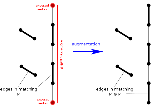
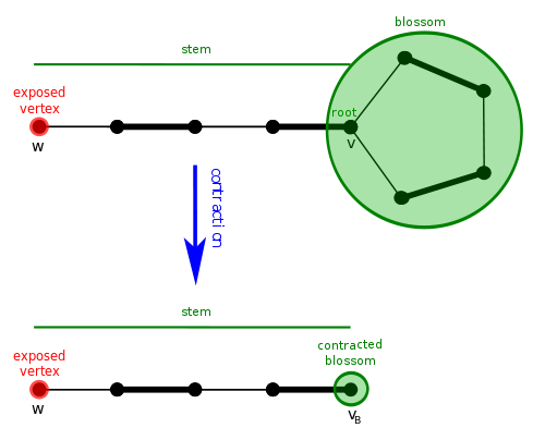
It will help if you are already familiar with bipartite matching. I will discuss the high level ideas of the algorithm, but my main focus will be on the tricky implementation details. So you may also want to read a supplementary resource like the Wikipedia page (from which I stole some pretty pictures).

Algorithm Overview

The blossom algorithm works by increasing the number of matched edges by one at a time until it cannot increase it further, then it stops. It's not as simple as just adding a new edge and keeping all the edges from previous iterations. If we did this, we might make a wrong decision and have a sub-optimal matching. Instead of simply searching for one new edge to add to the set, we should search for an augmenting path. This is a path where the edges alternate between being matched and unmatched. A vertex is called exposed if it is not adjacent to any matched edge. Another requirement of augmenting paths is that the endpoints should both be exposed. Also, it must be a simple path, meaning it cannot repeat any vertices.

If we find an augmenting path, we can easily increase the number of matched edges by $$$1$$$. We simply change all the matched edges to unmatched and all the unmatched edges to matched. An augmenting path has one more unmatched edge than matched edges, so it's correct. We can also easily see that it will still be a valid matching, i.e. no two matched edges will share a vertex. Ok, so augmenting paths are useful for increasing our matching, but are they guaranteed to exist if we don't have a maximum matching? Yes! In fact, consider $$$M_1$$$ to be the set of edges in our current matching and $$$M_2$$$ to be the set of edges in some maximum matching. Now, the symmetric difference $$$M_1\oplus M_2$$$ will be all the edges in exactly one of the two matchings. Based on the matching property, each vertex has degree $$$1$$$ or $$$2$$$. So each connected component must be a cycle or a path. Since we assume $$$M_2$$$ has more edges than $$$M_1$$$, there must be some connected component in $$$M_1\oplus M_2$$$ with more edges from $$$M_2$$$ than $$$M_1$$$. The only way this can happen is if one of the components is an augmenting path.

Great! Now all we have to do is figure out how to find an augmenting path in a matching, and we're done. Unfortunately, this is more difficult than it sounds. We might think of just using a DFS or BFS from exposed vertices, and ensuring that edges always alternate between matched and unmatched. For example, we could say each vertex $$$v$$$ has two versions $$$(v, 0)$$$ and $$$(v, 1)$$$. We can ensure that matched edges always go from version $$$1$$$ to $$$0$$$ and unmatched from $$$0$$$ to $$$1$$$. So, what's wrong? Won't we correctly find an alternating path of matched and unmatched edges, from one exposed vertex to another? The issue is that we are not ensuring the path is simple. This process could find a path that visits both $$$(v, 0)$$$ and $$$(v, 1)$$$ for some $$$v$$$. Then if you "flip" all the edges, $$$v$$$ would be adjacent to two matched edges, which is a violation. However, this simple DFS/BFS idea does work correctly in bipartite matching, and you might see it's equivalent to the algorithm you already know.

Blossoms

To deal with the problem of repeating vertices, we introduce the concept of blossoms. A blossom is simply a cycle of $$$2k+1$$$ edges, where $$$k$$$ of them are matched edges. This means there is exactly one "special" vertex $$$v$$$ in the cycle that isn't matched to another vertex in the cycle. Why do we care about blossoms? Because they create a situation where an alternating DFS/BFS could repeat a vertex.

Now that we know what they are, how does the blossom algorithm handle them? It contracts them. This means that we merge all vertices of the blossom into a single vertex, and continue searching for an augmenting path in the new graph.

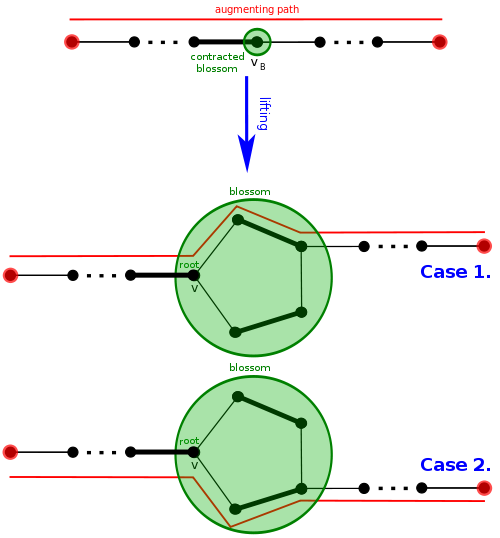
If we eventually find an augmenting path, we will have to lift the path back to our original graph. It can be shown that a graph has an augmenting path if and only if it has one after contracting a blossom. The concept of contracting blossoms and lifting an augmenting path makes it challenging to implement correctly. Remember, a contracted blossom can become a vertex in another blossom, so you can have blossoms inside blossoms inside blossoms! You should be experiencing headaches around now.

Let's see intuitively how an augmenting path can be lifted, effectively "undoing" a blossom contraction while keeping an augmenting path. Well, there should be an edge entering the blossom and then an edge leaving it. Since the path is alternating in the contracted graph, one of those two edges is matched. This means the "special" vertex $$$v$$$ of the blossom will be involved. Suppose $$$u$$$ is the vertex involved with the unmatched edge leaving the blossom. Let's go around the cycle between $$$u$$$ and $$$v$$$, but there are two ways, which do we take? Of course, it should be alternating, so we have exactly one correct choice.

Summary

In summary, the algorithm works like this. We repeat the following process until we fail to find an augmenting path, then return. We begin a graph search with DFS or BFS from the exposed vertices, ensuring that the paths alternate between matched and unmatched edges. If we see an edge to an unvisited node, we add it to our search forest. Otherwise if it's a visited node, there are three cases.

  1. The edge creates an odd cycle in the search tree. Here, we contract the blossom and continue our search.
  2. The edge connects two different search trees and forms an augmenting path. Here, we keep undoing the blossom contractions, lifting the augmenting path back to our original graph, and flip all the matched and unmatched edges.
  3. The edge creates neither case 1 nor case 2. Here, we do nothing and continue our search.

Implementation in $$$O(n^3)$$$

For the implementation, I will use an integer ID for each vertex and for each blossom. The vertices will be numbered from $$$0$$$ to $$$n-1$$$, and blossoms will start at $$$n$$$. Every blossom contraction gets rid of at least $$$3$$$ previous vertices/blossoms, so there can be at most $$$m:=\frac{3n}{2}$$$ IDs. Now, here is my organization of all the data:

  • mate: an array of length $$$n$$$. For each vertex u, if it's exposed we have mate[u] = -1, otherwise it will be the vertex matched to u.
  • b: for each blossom u, b[u] will be a list of all the vertices/blossoms that were contracted to form u. They will be listed in cyclic order, where the first vertex/blossom in the list will be the "special" one with an outgoing matched edge.
  • bl: an array of length $$$m$$$. For each vertex/blossom u, bl[u] will be the blossom immediately containing u. If u is not contracted inside of another blossom, then bl[u] = u.
  • p: an array of length $$$m$$$. For each vertex/blossom u, p[u] will be the parent vertex/blossom of u in the search forest. However, we will be a bit relaxed: we also allow it if p[u] is contracted inside the real parent, or even contracted multiple times, as long as the vertex/blossom at the top is the real parent in the contracted graph.
  • d: an array of length $$$m$$$. For each vertex/blossom u, d[u] will be a label/mark telling its status in the search forest. We will assign d[u] = 0 if it's unvisited, d[u] = 1 if it's an even depth from the root, and d[u] = 2 if it's an odd depth from the root.
  • g: a table of size $$$m\times m$$$, storing information about the unmatched edges. For each pair of vertices/blossoms $$$(u, v)$$$, then g[u][v] = -1 if there is no unmatched edge between them. Otherwise if there's an unmatched edge, then we will use this table entry to help us with lifting augmenting paths. When we're lifting a path through a blossom, we would like to know which vertices inside the blossom need to be connected. So if u is a blossom, then g[u][v] will store the vertex inside the blossom of u that connects to v. Otherwise if u is a vertex, then g[u][v] = u.

Structure

Now, we can define the structure and a couple helper functions add_edge and match. We use add_edge to create an unmatched edge, and match to change an unmatched edge to matched.

Structure

Trace Path to Root

We will want a function that traces the path to the root, where we only take vertices/blossoms in the contracted graph. This is done by repeatedly finding the blossom at the top of the bl chain, and following the parent pointers p.

The complexity of this function is $$$O(n)$$$.

Trace

Blossom Contraction

Let's say we found an edge between vertices $$$x$$$ and $$$y$$$ that creates a blossom in the search forest, and we need to contract it. Let's say that $$$c$$$ should be the ID of the new blossom, and we've constructed the paths from $$$x$$$ and $$$y$$$ to the root (call the paths vx and vy). First, we need to find the special vertex of the blossom, which is given by the lowest common ancestor of $$$x$$$ and $$$y$$$. So, we can say $$$r$$$ is the last common element of the vectors vx and vy, and delete everything above and including $$$r$$$.

Next, we should define b[c] to be the blossom vertices in cyclic order, starting at $$$r$$$. Simply append vx in reverse order, then vy in forward order. Finally, we should make the g table correct for the blossom c. Simply look at each vertex z in the blossom and each edge of z.

The complexity of this function is $$$O(n|b_c|)$$$ if the number of vertices/blossoms in $$$c$$$ is $$$|b_c|$$$.

Contract

Path Lifting

Let's say that we have an augmenting path in the contracted graph, and we want to lift it back to the original graph. The input will be a list of blossoms, where each one connects to the next, and we want to expand all of the blossoms except the last one, and return the list A of vertices.

The input list will work like a stack. If the top is a vertex, we will add it to the output and continue. Otherwise, we will replace the top blossom with the path of blossoms/vertices inside it such that it's still an alternating path. The variables represent the following information:

  • z: the top of the stack
  • w: the next element on the stack after z
  • i: the index in the b[z] list of the last vertex on our lifted path
  • j: the index in the b[z] list of the first vertex on our lifted path
  • dif: the direction we should advance i until j so that the path is correctly alternating.

As you can see, we use the g table to find the vertices/blossoms at the level below z. We also use the parity of the size of A to determine if the incoming edge is matched or unmatched.

The complexity of this function is $$$O(n)$$$.

Lift

Putting it all Together

Now that we have the subroutines, let's implement the whole algorithm. First, the algorithm will repeatedly search for augmenting paths until we can't find one and return. So we have one big outer loop to count the number of edges in our matching. Next, to start an iteration we reset all our variables, and assume the g table is correct for the vertices. We will use a BFS-like process for the search forest, but something like DFS should also work. We look for all the exposed vertices and add them to the queue. The variable c will be used to count the total number of vertex/blossom objects, and we'll increment it with each blossom contraction.

When we dequeue a vertex $$$x$$$, assuming it's not contained in another blossom, we look at all unmatched edges leaving it. Say we're looking at an edge to another vertex $$$y$$$. There are several cases:

  1. The vertex $$$y$$$ is not visited. In this case, we will mark $$$y$$$ and its mate as visited, and add mate[y] to the queue.
  2. The vertex $$$y$$$ is visited and has an odd distance to the root. In this case, we should do nothing.
  3. The vertex $$$y$$$ is visited and has an even distance to the root. Here, we should trace the paths from $$$x$$$ and $$$y$$$ to the root to determine if this event is a blossom contraction or an augmenting path. In either case, we should break from the inner loop.

Let's analyze the time complexity. First, each iteration increases the number of matched edges by $$$1$$$ and so there can be at most $$$n/2$$$ iterations overall. The basic BFS operations will clearly take $$$O(n^2)$$$ time since each vertex appears in the queue at most once, and each dequeued element looks at all other vertices. An augmenting path is found at most once in an iteration, and it takes $$$O(n)$$$ time. A blossom contraction takes $$$O(n |b_c|)$$$ time, and each vertex/blossom will belong to at most one immediate blossom, so the overall time in an iteration from blossom contractions is $$$O(n^2)$$$. Since each iteration takes $$$O(n^2)$$$ time and there are $$$O(n)$$$ iterations overall, we see that the algorithm takes $$$O(n^3)$$$ time.

Solve

I've tested my implementation on these two sites. If you want to do further testing/benchmarking, feel free, and let me know if you find any issues.

Full text and comments »

  • Vote: I like it
  • +384
  • Vote: I do not like it

By Monogon, history, 4 years ago, In English

omg hi!

I will add implementations soon.

UPD: Implementations are added

1504A - Déjà Vu

Tutorial

Implementation

1504B - Flip the Bits

Tutorial

Implementation

1504C - Balance the Bits

Tutorial

Implementation

1504D - 3-Coloring

Tutorial

Implementation

1504E - Travelling Salesman Problem

Tutorial

Implementation 1

Implementation 2

1504F - Flip the Cards

Tutorial

Implementation

1503E - 2-Coloring

Tutorial

Implementation

1503F - Balance the Cards

Tutorial

Implementation

Full text and comments »

  • Vote: I like it
  • +566
  • Vote: I do not like it

By Monogon, history, 4 years ago, In English

omg hi!

I am pleased to invite you to participate in Codeforces Round 712 (Div. 1) and Codeforces Round 712 (Div. 2)! You will be given 6 problems and 2 hours 15 minutes to solve them. I'm happy to announce the theme of this round is déjà vu!

I would like to thank the following people:

Make sure you read all problems, and I'm happy to announce the theme of this round is déjà vu! Good luck, have fun!

The score distribution will be announced immediately because you deserve it ❤️:

Div. 1: 750 — 1000 — 1250 — 1750 — 2500 — 4000

Div. 2: 500 — 1000 — 1750 — 2000 — 2250 — 3000

UPD: Editorial

Full text and comments »

  • Vote: I like it
  • +2866
  • Vote: I do not like it

By Monogon, history, 4 years ago, In English

What's a Voronoi Diagram?

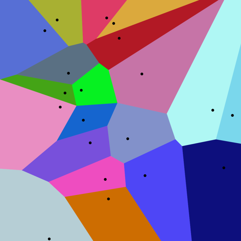
Given a set $$$S$$$ of $$$n$$$ points in the 2D plane, the Voronoi diagram is a partition of the plane into regions. The region associated with a point $$$p\in S$$$ contains precisely the points $$$q$$$ such that $$$q$$$ is closer to $$$p$$$ than any other point in $$$S$$$. In other words, a point $$$q$$$ belongs to the region of its nearest neighbor.

The Voronoi diagram can be represented by the planar graph of boundaries between regions. A vertex in this graph is where three or more segments meet (or a point at infinity), and an edge is a segment connecting two of these vertices. The way the regions were defined, we see that a segment contains the points equidistant to two points in $$$S$$$, so it is part of their perpendicular bisector. Similarly, a Voronoi vertex is equidistant to three or more vertices in $$$S$$$, so it is their circumcenter. Recall that the circumcenter is the intersection of perpendicular bisectors.

What's a Delaunay Triangulation?

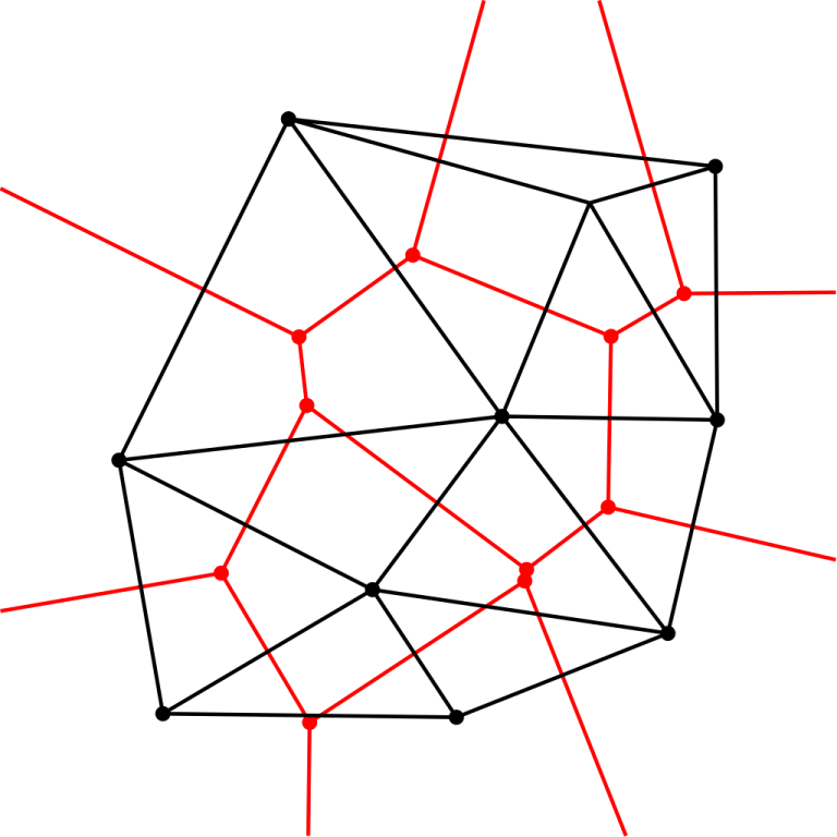
The Delaunay triangulation is the dual graph of the Voronoi diagram. That is, a Voronoi vertex is a Delaunay face and a Delaunay vertex is a Voronoi region. A Delaunay edge connects two points if and only if their corresponding Voronoi regions share a border.

In the following image, the set $$$S$$$ corresponds to the black points. The red vertices and edges are the Voronoi diagram. The black points and edges are the Delaunay triangulation.

The Delaunay triangulation only involves edges between existing points, while the Voronoi diagram creates new vertices and needs a way to represent edges going infinitely in one direction. For this reason, it is often more convenient to compute the Delaunay triangulation and only convert to the Voronoi diagram if needed.

Why are these useful?

The definition of the Voronoi diagram immediately shows signs of applications. Given a set $$$S$$$ of $$$n$$$ points and $$$m$$$ query points $$$p_1,\ldots, p_m$$$, we can answer for each query point, its nearest neighbor in $$$S$$$. This can be done in $$$O((n + q)\log(n+q))$$$ offline by sweeping the Voronoi diagram and query points. Or it can be done online with persistent data structures.

Other than this, the Delaunay triangulation has many amazing properties of its own that can make it extremely useful for solving problems.

  • For each Delaunay triangle, its circumcircle does not strictly contain any points in $$$S$$$. (In fact, you can also consider this the defining property of Delaunay triangulation)
  • The number of Delaunay edges is at most $$$3n-6$$$, so there is hope for an efficient construction.
  • Each point $$$p\in S$$$ is adjacent to its nearest neighbor with a Delaunay edge.
  • The Delaunay triangulation maximizes the minimum angle in the triangles among all possible triangulations.
  • The Euclidean minimum spanning tree is a subset of Delaunay edges.

Degenerate Cases

Because this is geometry, there are some degenerate cases I have hidden from you up to this point. The first case is when all the points in $$$S$$$ are contained in a line. In this case, the Voronoi diagram has all edges connecting two points at infinity, and the Voronoi diagram is disconnected (in all other cases it's connected). Also in this case, the dual graph is no longer a triangulation. We may still decide to represent it by the path of edges connecting the points.

Another nasty case is co-circular points. Here, there are Voronoi vertices where more than three segments intersect. In this case, the dual graph has a face with more than three sides. However, we want it to be a triangulation, so we can also say that any triangulation of such faces is valid, and we will allow non-unique Delaunay triangulations.

Algorithms

Many algorithms exist to compute the Delaunay triangulation and/or Voronoi diagram of a set of points. Each have their advantages and disadvantages.

Flip Algorithms

In this approach, you start with an arbitrary triangulation of the points. Then you repeatedly fix adjacent triangle pairs until the triangulation has the Delaunay property. The main advantage of this method is its simplicity: an arbitrary triangulation can be constructed with an incremental convex hull algorithm, and the disadvantage is that it could require $$$\Omega(n^2)$$$ flips in the worst case.

Incremental Algorithms

In this approach, you always maintain the Delaunay triangulation of a subset of the points and insert the points one at a time. When a point is inserted, you should delete all triangles whose circumcircle contains the newly added point. After deleting this connected set of triangles, you should repair the face it exposes. For each edge in this exposed face, you should add a triangle with that edge and the new point. This gives the straightforward $$$O(n^2)$$$ Bowyer-Watson algorithm.

If we insert the points in a random order, we can significantly reduce the number of triangle insertions and deletions. But to get expected $$$O(n\log n)$$$ runtime, we would need to avoid processing all the unaffected triangles. And this makes the implementation far more challenging. We need to maintain a search structure of the triangles in order to locate which one contains the new point.

The advantage of this method is that it achieves expected $$$O(n\log n)$$$ runtime with only integer computations, and the construction is online. The disadvantage is that it has a bad constant, isn't deterministic, and the triangle search structure can make for a tricky implementation.

Divide and Conquer

The divide and conquer algorithm first sorts the points by $$$x$$$-coordinate. Then it splits the points into two sets, recursively computes their Delaunay triangulations, and merges them together. As long as you can perform the merge in $$$O(n)$$$ time, the overall algorithm is $$$O(n\log n)$$$. When merging the triangulations, it is actually quite hard to keep track of the important adjacency information. The most popular strategy is perhaps the Quad-Edge data structure.

The advantage is that this gives a deterministic $$$O(n\log n)$$$ algorithm with only integer computations. The disadvantage is the complexity of the quad-edge data structure and the costly memory usage that comes with it.

3D Convex Hull Reduction

An interesting fact is that the problem of Delaunay triangulation can be reduced to 3D convex hull. If for each point $$$(x,y)$$$ we also give it the $$$z$$$-coordinate $$$x^2+y^2$$$ and compute the 3D convex hull, then the downward-facing convex hull faces correspond exactly to the Delaunay triangles. The advantage is that if you happen to have a good 3D convex hull implementation, you get Delaunay triangulation for free. The disadvantages are that $$$O(n\log n)$$$ 3D convex hull is a whole beast of its own, and the large $$$z$$$-coordinates will exacerbate precision and overflow errors in the 3D convex hull implementation. The main strategies for 3D convex hull are incremental and divide-and-conquer algorithms, which are only more complicated than their counterparts in the special case of Delaunay triangulation.

My previous blog on 3D convex hull gave an $$$O(n\log n)$$$ randomized incremental implementation, but it turns out to have quite a bad constant for practical use.

Fortune's Algorithm

In this blog, I will focus on Fortune's Algorithm. It takes a sweep-line approach to the problem, and achieves a deterministic $$$O(n\log n)$$$ time complexity. The main disadvantage is that computations are done with floating points instead of integers, opening up the door to precision errors. However, keep in mind that the algorithms using only integers have a risk of integer overflow even on reasonably small constraints.

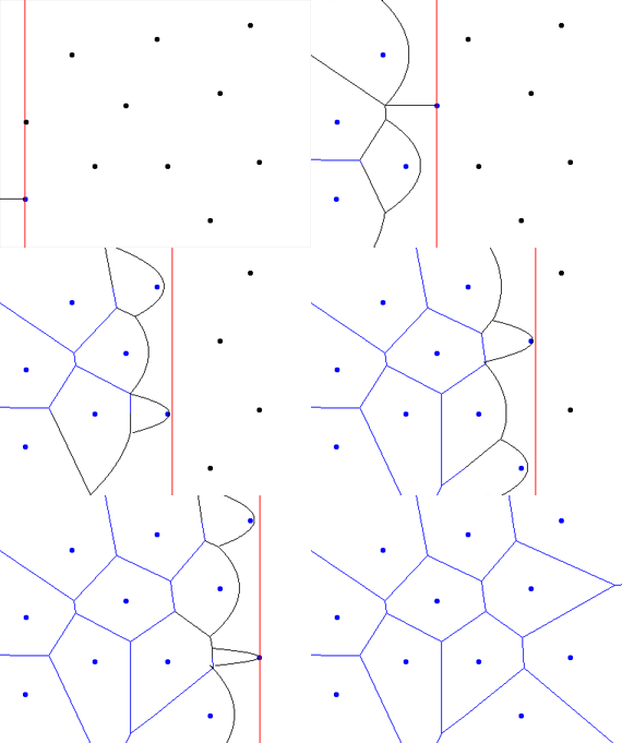
The main challenge in designing a sweep-line algorithm for Voronoi diagrams is that a point after the sweep-line can affect the diagram before the sweep-line. That is, if the sweep-line denotes the discovery time of a point, we cannot know the entire Voronoi diagram before the sweep-line. The way Fortune's algorithm overcomes this challenge is by maintaining the Voronoi diagram only for the area we can be certain about, regardless of what points lie after the sweep-line.

Now, which points can be affected by what lies past the sweep-line? Well, such a point must be closer to the sweep-line than to any point in $$$S$$$ to the left of the sweep-line. Recall that the set of points equidistant to a point and a line is given by a parabola, where the point is called the focus and the line is called the directrix. If the focus is a point $$$p\in S$$$ to the left of the sweep-line and the directrix is the sweep-line, then everything to the left of this parabola we can be certain of its region. Now, if we make such a parabola for every point $$$p\in S$$$ to the left of the sweep-line, everything to the right of all parabolas is precisely the uncertain region. The boundary of the certainty and uncertainty regions is called the beach line, consisting of parabolic arcs.

We are ready to understand Fortune's algorithm abstractly. We scan a sweep-line from left to right, maintaining the combinatorial structure of the beach line. The parabolas are only for visual aid, and the ordered list of foci is what is actually stored. As points get added and parabolic arcs shrink to length $$$0$$$, these events tell us precisely the structure of the Voronoi diagram and Delaunay triangulation.

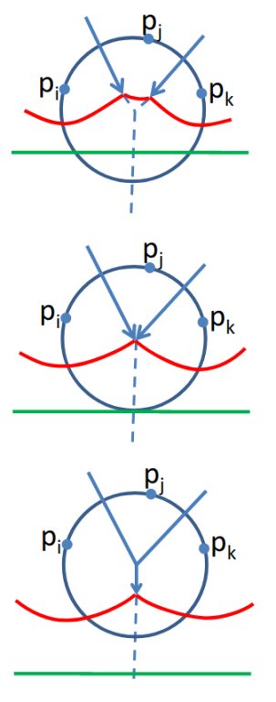
There are two types of events which change the beach line structure: point events and vertex events.

Point Events

In a point event, the sweep-line discovers a point $$$p\in S$$$ and inserts its parabolic arc into the beach line. In order to do this efficiently, we need to search for where it belongs in the beach line. Then it will split the arc it sees into two. An example of a point event is shown below (here the sweep-line goes from top to bottom instead).

Vertex Events

In a vertex event, a parabolic arc disappears from the beach line, corresponding to a Voronoi vertex. To handle a vertex event, we simply remove the point whose arc length shrinks to length $$$0$$$. Such an event is generated dynamically by a triple of points adjacent on the beach line. Every time we modify the beach line, we update the relevant points for their vertex events. To compute the time a vertex event should be handled, we take the circumcircle of the three points generating the event. The rightmost point of the circumcircle is the time we should process this event.

Summary

In summary, the algorithm maintains a priority queue of events. Initially, we push all point events into the priority queue. When processing a point event, we find the correct arc in the beach line, split it up, add the new point, and add new vertex events if needed. When processing a vertex event, we add the generating triple as a Delaunay triangle, remove the arc that should disappear, and add new vertex events if needed.

Fortune's Algorithm Implementation

My code doesn't work when two points have the same $$$x$$$ coordinate. This is handled simply by rotating all input points by $$$1$$$ radian and praying to the geometry gods.

Implementation

Example Problems

Panda Preserve solution
Caravans solution
Good Manners solution

Resources

Full text and comments »

  • Vote: I like it
  • +499
  • Vote: I do not like it

By Monogon, history, 4 years ago, In English

I hope you enjoyed the problems! Implementations will be added soon.

UPD: Implementations are added!

1450A - Avoid Trygub

Tutorial

Implementation

1450B - Balls of Steel

Tutorial

Implementation

1450C1 - Errich-Tac-Toe (Easy Version)

Tutorial

Implementation

1450C2 - Errich-Tac-Toe (Hard Version)

Tutorial

Implementation

1450D - Rating Compression

Tutorial

Implementation

1450E - Capitalism

Tutorial

Implementation

1450F - The Struggling Contestant

Tutorial

Implementation

1450G - Communism

Tutorial

Implementation

1450H1 - Multithreading (Easy Version)

Tutorial

Implementation

1450H2 - Multithreading (Hard Version)

Tutorial

Implementation

Full text and comments »

  • Vote: I like it
  • +382
  • Vote: I do not like it

By Monogon, history, 4 years ago, In English

¡Buenos días! (That's Spanish for "what's up homies")

On Dec/06/2020 17:35 (Moscow time) we will host Codeforces Global Round 12.

It is the sixth round of a 2020 series of Codeforces Global Rounds. The rounds are open and rated for everybody.

The prizes for this round:

  • 30 best participants get a t-shirt.
  • 20 t-shirts are randomly distributed among those with ranks between 31 and 500, inclusive.

The prizes for the 6-round series in 2020:

  • In each round top-100 participants get points according to the table.
  • The final result for each participant is equal to the sum of points he gets in the four rounds he placed the highest.
  • The best 20 participants over all series get sweatshirts and place certificates.

Thanks to XTX, which in 2020 supported the global rounds initiative!

The problems were written and prepared by smart Cuban Devil and stupid Americans fivefourthreeone and Monogon.

We would like to distribute our thanks equally to the following people who made this round possible.

You will have 3 hours to solve 8 problems (and 2 subtasks). If you want to lose rating, then we encourage you not to read all the problems.

May rating be distributed from each according to his ability, to each according to his needs!

UPD: Here's the score distribution. Good luck, have fun!

$$$500-750-(1000+750)-1750-2500-2750-3750-(2750+1750)$$$

UPD: Hope you enjoyed the problems! Editorial is posted.

UPD: System testing finished, congrats to the winners!

  1. Benq
  2. tourist
  3. jiangly
  4. IZONE
  5. ecnerwala
  6. Um_nik
  7. ksun48
  8. 244mhq
  9. maroonrk
  10. yosupo

Full text and comments »

Announcement of Codeforces Global Round 12
  • Vote: I like it
  • +1239
  • Vote: I do not like it

By Monogon, history, 4 years ago, In English

The upcoming round has an unusual starting time. In order to keep my performance slightly less bad than usual, I will apply the "destroy my sleep schedule" strategy. For some unknown reason I have decided to document this by beginning my streaming career.

https://www.twitch.tv/monogoncoding

Full text and comments »

  • Vote: I like it
  • +266
  • Vote: I do not like it

By Monogon, history, 4 years ago, In English

Randomization is known to be a powerful algorithmic technique, and I want to start a discussion about it specifically in the context of competitive programming. What extra considerations should we make about how online judges work when analyzing our randomized algorithms, and approving such problems for an official contest? In particular, I want to discuss algorithms whose running times are uncertain.

Let's say that the running time of an algorithm is a random variable $$$X$$$. Typically, we might say the algorithm is acceptable if the expected running time is a fraction of the time limit: $$$E(X)=T/k$$$. With Markov's inequality, we can say $$$P(X>T)\le 1/k$$$. That is, the probability of failing a test case due to timeout is at most $$$1/k$$$.

TLE Trick

Online judges usually run your program a few times before giving the Time Limit Exceeded verdict. This fact is known to help randomized algorithms, as mentioned here: https://codeforces.me/blog/entry/78817

Let's apply this in the context of random running times. If your program is run $$$n$$$ times, the actual probability of failing a test case is at most $$$1/k^n$$$. If there are $$$m$$$ test cases total, the probability of failing at least one of the test cases is $$$1-(1-1/k^n)^m$$$

Solving for $$$k$$$

Let's suppose we call a program acceptable if its probability of failure is at most $$$p$$$. Then we are interested in what the constant $$$k$$$ should be in order to be confident of success.

$$$k\ge \left[ 1-(1-p)^{1/m}\right]^{-1/n}$$$

Let's plug in some values. Suppose there are $$$m=200$$$ test cases, your program gets $$$n=3$$$ chances per test case, and we can tolerate a failure probability of $$$p=10^{-3}$$$. Then we should require $$$k\approx 58.47$$$, which is quite a considerable constant factor that we should be careful about when making randomized solutions.

Future Directions

If we make extra assumptions on the distribution of $$$X$$$ that apply widely to randomized algorithms, can we be confident with a much smaller value of $$$k$$$? What will the analysis look like on some specific cases like treaps? I'm interested to hear your thoughts.

Full text and comments »

  • Vote: I like it
  • +14
  • Vote: I do not like it

By Monogon, history, 4 years ago, In English

I hope everyone enjoyed the contest!

UPD: Added implementations for all problems.

1405A - Permutation Forgery

Author: antontrygubO_o

Tutorial

Implementation

1405B - Array Cancellation

Author: hugopm

Tutorial

Implementation

1405C - Balanced Bitstring

Author: Kuroni

Tutorial

Implementation

1405D - Tree Tag

Author: Merripium

Tutorial

Implementation

1405E - Fixed Point Removal

Author: hugopm

Tutorial

Implementation

1404D - Game of Pairs

Author: Ari

Tutorial

Implementation

1404E - Bricks

Author: Monogon

Tutorial

Implementation

Full text and comments »

  • Vote: I like it
  • +421
  • Vote: I do not like it

By Monogon, history, 4 years ago, In English

Warning: The following contains graphic depictions of geometry, precision errors, and degenerate cases. Viewer discretion is advised.

Prerequisites

I assume the reader is familiar with:

  • 2D Convex Hulls
  • 3D Vector Operations (dot and cross products)

Introduction

Recall that in the 2D convex hull problem, you are given a set of 2D points, and you must compute the smallest convex polygon containing all the given points. By convex, we mean that for any two points $$$A$$$ and $$$B$$$ inside the polygon, the entire line segment $$$AB$$$ is also inside the polygon.

The problem in 3D is completely analogous. You are given $$$n$$$ 3D points, and you must compute the smallest convex polyhedron containing all the given points. Similarly, a polyhedron is convex if for any two points $$$A$$$ and $$$B$$$ inside the polyhedron, the line segment $$$AB$$$ is also inside the polyhedron.

In the 2D case, it is more obvious what the output is. We can simply output a circular list of vertices on the boundary of the polygon. But how do we represent a polyhedron? Well, we can represent it as a list of triangular faces. A non-triangular face can always be divided into triangles, so this requirement isn't limiting.

In the 2D case, there are some degenerate cases that are easy to miss if you're not careful. For example, if there are 3 collinear points, the polygon might have two adjacent sides of the same slope, or you might combine them into one segment. Or if two points have the same $$$x$$$ coordinate, you need to handle this carefully when sorting the points by $$$x$$$ coordinate. Or if all the points are on the same line, then the convex hull isn't even a non-degenerate polygon!

Now, degenerate cases are bad enough with two dimensions. When you enter the third dimension, it only gets worse. What if four points lie on the same plane? Since we are requiring triangular faces, we could triangulate this in multiple ways. Or maybe we could choose to have one triangle of three points and the forth point lies inside this triangle, so we ignore it. What if all the points are on the same line? Or on the same plane even? Then the convex hull isn't a non-degenerate polyhedron. I will ignore such degenerate cases for now, and revisit them when applicable.

Brute Force Algorithm in $$$O(n^4)$$$

Suppose that $$$n$$$ is very small, and we are guaranteed that no four points are coplanar. Then how can we compute the 3D convex hull in the dumbest way possible?

We could simply consider every triplet of three points $$$(\vec{a}, \vec{b}, \vec{c})$$$, and check if they create a triangular face on the convex hull. In order for it to be a face, the remaining points must "see" the same side of the triangle. In other words, if we consider the plane containing this triangle, the remaining points should lie on the same side of the plane. To compute which side of a plane a point $$$\vec{p}$$$ is on, we can first take a vector $$$\vec{q}=(\vec{b}-\vec{a})\times (\vec{c}-\vec{a})$$$ orthogonal to the plane.

Then the sign of $$$(\vec{p}-\vec{a})\cdot \vec{q}$$$ tells us the side of the plane. In particular, a result of $$$0$$$ tells us that $$$\vec{p}$$$ lies on the plane.

For each triplet, we perform this check with all points, so the total time complexity is $$$O(n^4)$$$. Because of its simplicity, this should be the approach when the constraints allow it. And by examining the brute force case, we learned how to perform the most fundamental operation in any 3D convex hull algorithm: checking which side of a plane a point is on.

Incremental Algorithm in $$$O(n^2)$$$

Now we want a more practical algorithm. The strategy of the incremental algorithm is to build the convex hull for the first $$$i$$$ points, as $$$i$$$ goes from $$$1$$$ to $$$n$$$. All we have to do is figure out how to update the convex hull in order to accommodate one new point.

Let's start by making an analogy with the 2D convex hull. Suppose we currently have the convex hull of the first $$$i-1$$$ points, and we wish to add the $$$i$$$-th point. Well, if the point is already inside the hull, we should do nothing. Otherwise, let's pretend we are looking at the polygon from the perspective of the $$$i$$$-th point. We should delete all line segments it can see, and add two new line segments: one from the new point to each of the extreme points.

A similar thing happens in the 3D case. If a point is already inside the polyhedron, we simply do nothing. Otherwise, we delete all faces the new point can see. But what's less obvious is what we should add. Well, we've left the polyhedron with a connected set of faces removed. This exposes a cycle of edges. For each of these exposed edges, we should create a new face with the new point and that edge. Effectively, we create a cone of faces to repair the opening.

Now, let's analyze the time complexity. For each iteration, we process all faces of the hull in that iteration. And it can be proven that the number of faces is at most $$$O(n)$$$. For the proof, we use Euler's Formula. It states that for any polyhedron with $$$V$$$ vertices, $$$E$$$ edges, and $$$F$$$ faces, $$$V-E+F=2$$$. All faces are triangles, so we can substitute $$$E=3F/2$$$ since each face has $$$3$$$ edges, and we count each edge twice for the $$$2$$$ faces it touches. Then we have $$$V-F/2=2$$$ and $$$F=2V-4=O(n)$$$. Since we process $$$O(n)$$$ faces in $$$O(n)$$$ iterations, the overall time complexity is $$$O(n^2)$$$.

Implementation

Clarkson-Shor Algorithm in $$$O(n\log n)$$$

There exist deterministic algorithms to compute the 3D convex hull in $$$O(n\log n)$$$ time. Most famously, there is a divide-and-conquer algorithm that solves it, but it is notoriously difficult to implement correctly. But don't lose hope! There is also a randomized algorithm based on the same incremental strategy, which takes $$$O(n\log n)$$$ time in expectation if the points are added in random order.

Unfortunately, we can't just shuffle the points, run the usual incremental algorithm, and call it a day. In order to achieve $$$O(n\log n)$$$, we should eliminate extra work of processing faces invisible to the new point. How can we do this? Well, before we checked for each point, which faces it can see. Instead, we will maintain for each point a list of faces it can see. Then when a face is created, we add it to the lists of all points that will be able to see it.

"Wait a minute," I hear you ask, "isn't this still $$$O(n^2)$$$ because you still process the same thing for each face-point pair, just in a different order?" The answer is yes, we're still in $$$O(n^2)$$$ territory. But, using some cleverness we can avoid checking with every future point every time. The key idea is that a new face $$$F$$$ is attached to a preexisting edge $$$e$$$, and a point $$$p$$$ can see $$$F$$$ only if it was able to see one of the two faces of $$$e$$$. Instead of checking with all future points, we will only check the points in the lists associated with these two faces. Unfortunately, this requires more work to implement. This time, we need to start caring about how the faces touch each other in order to find these two lists.

Precision Errors and Degenerate Cases

The only potential source for precision error is our check of which side of a plane a point is on. If all coordinates are integers, then our computations will stay as integers. If it overflows on 64-bit integer types, we can convert to floating points for computations, and set $$$\epsilon=0.5$$$. Note that if the coordinates are at most $$$X,Y,Z$$$ in absolute value (in the $$$x$$$, $$$y$$$, and $$$z$$$ directions, respectively), our computations are on the order of $$$XYZ$$$. Use this to determine whether it will overflow on integers or find what you should set $$$\epsilon$$$ to. Or just try every possible $$$\epsilon$$$ until it works.

To handle degenerate cases, we should make sure that the first $$$4$$$ points are not coplanar. If all the $$$n$$$ points do not lie in the same plane, we can find $$$4$$$ such points and move them to the beginning. Once this is taken care of, the only real degenerate case remaining is when we need to decide if a face is visible to a point in the same plane. I made the decision to consider the face invisible in such a case. This ensures that the algorithm won't unnecessarily subdivide faces. However, it is still possible that the algorithm can have non-unique output depending on the order the points are processed. This is inevitable since there is not a unique way to triangulate faces in degenerate cases. If we want to, though, we can combine adjacent coplanar faces afterward.

To my knowledge, the Clarkson-Shor algorithm doesn't make any guarantees about $$$O(n\log n)$$$ performance when there are degenerate cases. I think by considering coplanar faces invisible, we are safe. But if anyone has a nasty test case against it, I'm interested to hear it.

Here is my implementation of the $$$O(n\log n)$$$ algorithm with full handling of degenerate cases (I hope). If anyone finds bugs or ways to improve the efficiency and/or readability of this implementation, please let me know!

Implementation

Application: Delaunay Triangulation and Voronoi Diagrams

Suppose we have $$$n$$$ 2D points $$$p_1,\ldots,p_n$$$. We may want to answer queries of the form "Which point is closest to $$$q_i$$$?" for $$$m$$$ points $$$q_1,\ldots,q_m$$$.

The Voronoi diagram divides the plane into $$$n$$$ regions in a way that can answer these kinds of queries. It is defined so that the region corresponding to the point $$$i$$$ consists of all points closer to $$$p_i$$$ than any other of the $$$n$$$ points. That is, it's the region of points whose nearest neighbor is $$$p_i$$$. The Voronoi diagram can be represented by $$$O(n)$$$ line segments that border the regions (some line segments will extend to a point at infinity). We can answer our queries by sorting all line segments and queries, and performing a sweep line.

The dual of the Voronoi diagram is called the Delaunay Triangulation. It is the graph that connects two points if their Voronoi cells share a boundary edge. Conversely, the points of a Voronoi diagram are the circumcenters of Delaunay triangles, and an edge in the Voronoi diagram connects the circumcircles of two adjacent Delaunay triangles.

The Delaunay triangulation has several nice properties that come in handy. Most notably, the Euclidean minimum spanning tree consists of a subset of Delaunay edges. A nice consequence of implementing 3D convex hull is that we get Delaunay triangulation for free. We can simply map each point $$$(x,y)$$$ into a 3D point $$$(x,y,x^2+y^2)$$$. Then the downward-facing triangles of the 3D convex hull are precisely the Delaunay triangles. The proof is left as an exercise to the reader.

Resources

Practice Problems

Full text and comments »

  • Vote: I like it
  • +393
  • Vote: I do not like it

By Monogon, history, 4 years ago, In English

I hope you enjoyed the contest! I will add implementations later.

UPD I've added implementations.

1382A - Common Subsequence

Tutorial

Implementation

1382B - Sequential Nim

Tutorial

Implementation

1382C1 - Prefix Flip (Easy Version)

Tutorial

Implementation 1 Implementation 2

1382C2 - Prefix Flip (Hard Version)

Tutorial

Implementation 1 Implementation 2

1382D - Unmerge

Tutorial

Implementation

1382E - Mastermind

Tutorial

Implementation

1381D - The Majestic Brown Tree Snake

Tutorial

Implementation

1381E - Origami

Tutorial

Implementation

Full text and comments »

  • Vote: I like it
  • +497
  • Vote: I do not like it

By Monogon, history, 5 years ago, In English

Hello, Codeforces!

I'm very glad to invite you to Codeforces Round 658 (Div. 1) and Codeforces Round 658 (Div. 2). This contest will take place on Jul/21/2020 17:35 (Moscow time). In both divisions, you will have 2 hours to solve 5 problems (and one subtask). The score distribution will be announced closer to the start of the round.

Huge thanks to:

I've worked hard to ensure the pretests are short and the statements are strong. Remember to only read the problems that you can solve, and may you have the best of luck!

Because I know you all have so many questions, I have compiled an FAQueue

  • Q: Is it rated?
  • A: Yes

UPD Here is the score distribution:

Div. 2: 500 — 1250 — (1000 + 1000) — 2250 — 3000

Div. 1: (500 + 500) — 1500 — 2000 — 2500 — 3000

UPD Editorial

UPD I filled in the answer to the FAQ. Also, congrats to the winners!

Div. 2:

  1. badger_champion

  2. Mai_madarchod_hu

  3. rulai

  4. Vimmer

  5. niynip

Div. 1:

  1. Benq

  2. Um_nik

  3. KAN

  4. Petr

  5. ksun48

Full text and comments »

  • Vote: I like it
  • +2085
  • Vote: I do not like it

By Monogon, history, 5 years ago, In English

Hello, Codeforces!

I'm very glad to invite you to Codeforces Round 639 (Div. 1) and Codeforces Round 639 (Div. 2). This contest will take place on May/06/2020 17:35 (Moscow time). In both divisions, you will have 2 hours 15 minutes to solve 6 problems. The score distribution will be announced closer to the start of the contest.

Of course, this round would not be possible without the help of many people, who I'd like to thank:

I've done my best to write clear problem statements and strong pretests. Don't forget to read all problems, and I hope you enjoy the round. Good luck!

Because I know you all have so many questions, I have compiled an FAQ:

  • Q: Is it rated?
  • A: Yes.

UPD

Here is the score distribution.

Div. 1: 500 — 1000 — 1500 — 1750 — 2500 — 2500

Div. 2: 500 — 1000 — 1500 — 2000 — 2500 — 2750

UPD Unfortunately, this contest is delayed due to problems in the Codeforces system. It is temporarily scheduled, but I will update this announcement when a final decision on scheduling has been made. It is sad that my contest is delayed, but let's be grateful that the issue was detected early instead of arising in the middle of the round. On the bright side, this may be the earliest announced score distribution in Codeforces history.

UPD The final decision on scheduling is to keep it as is. The contest will take place on May/06/2020 17:35 (Moscow time).

UPD Unfortunately due to the long queue and other issues, the contest is unrated. There was also a bug that gave us trouble in answering your questions. I'm sorry if you asked a question that went unanswered for a long time. I promise we did our best to answer as many questions as we could! Despite all the problems, I hope you enjoyed the problemset!

UPD Editorial

Full text and comments »

  • Vote: I like it
  • +2313
  • Vote: I do not like it

By Monogon, history, 5 years ago, In English

1345A - Puzzle Pieces

Tutorial

1345B - Card Constructions

Tutorial

1345C - Hilbert's Hotel

Tutorial

1345D - Monopole Magnets

Tutorial

1345E - Quantifier Question

Tutorial

1345F - Résumé Review

Tutorial

1344E - Train Tracks

Tutorial

1344F - Piet's Palette

Tutorial

Full text and comments »

  • Vote: I like it
  • +586
  • Vote: I do not like it