430A - Points and Segments (easy)

The problem asks you to output “-1” if there is no solution. A natural question is now: “when there is no solution”? Try to come up with a test like this!

After some analysis, you’ll see anyhow we draw the points and the lines, there will always be a solution. By manually solving small cases, you might already have found the pattern. But for now, let’s assume anyhow we draw points and lines, there will always be a solution. Let’s have a fixed set of points. Then, anyhow we draw a line, there should still be a solution. So, we need to find a coloring of points, such as for every line, |number of red points which belong to it – number of blue points which belong to it| <= 1.

Suppose anytime you color a point with red you assign it +1 value. Also, anytime you color it with blue you assign it -1 value. Then, for a segment, the drawing is good if S = sum of values assigned to points that belong to segment is between -1 and 1 (in other words |S| <= 1). Let’s sort points increasing by abscissa. It’s useful because now, for a segment, there will be a contiguous range of points that belong to that segment. For example, suppose my current segment is [3, 7] and the initial set of points was {4, 1, 5, 2, 8, 7}. Initially, points that belong to the segment would be first, third and sixth. Let’s sort the points by abscissa. It looks like {1, 2, 4, 5, 7, 8}. You can see now there is a contiguous range of points that belongs to [3, 7] segment: more exactly third, fourth and fifth.

We reduced problem to: given an array, assign it either +1 or -1 values such as, for each subarray (contiguous range), the sum S of subarray’s elements follows the condition |S| <= 1. Before reading on, try to come up with an example by yourself.

My solution uses the pattern: +1 -1 +1 -1 +1 -1 ... Each subarray of it will have sum of its elements either -1, 0 or 1. How to proof it? When dealing with sums of subarrays, a good idea is to use partial sums. Denote sum[i] = x[1] + x[2] + ... + x[i]. Then, sum of a subarray [x, y] is sum[y] – sum[x – 1]. Partial sums for the pattern looks like: 1 0 1 0 1 0 .... Hence, there are 4 possible cases:

1/ sum[x – 1] = 0 and sum[y] = 0. sum[y] – sum[x – 1] = 0

2/ sum[x – 1] = 1 and sum[y] = 1. sum[y] – sum[x – 1] = 0

3/ sum[x – 1] = 0 and sum[y] = 1. sum[y] – sum[x – 1] = 1

4/ sum[x – 1] = 1 and sum[y] = 0. sum[y] – sum[x – 1] = -1

Hence, each subarray sum is either -1, 0 or 1. So, general algorithm looks like: sort points by abscissa, assign them red, blue, red, blue, ... and then sort them back by original order and print the colors.

430B - Balls Game

This is an implementation problem. There is not so much to explain. Perhaps the trick at implementation problems is to divide code into smaller subproblems, easy to code and then put them together. I don’t know if this is the universally truth, but this is how I approach them. Here, there are two main parts: the part when you insert a ball between 2 balls and the part when you see how many balls are destroyed after the move. We can keep an array a[] with initial configuration of balls, then for each insertion create an array b[] with current configuration after the insertion. If my ball is inserted after position pos, b is something like this: b = a[1....pos] + {my_ball} + a[pos+1....n].

For now we have array b[] and we need to know how many balls will disappear. The problem statement gives us an important clue: no 3 balls will initially have the same color. This means, any time, at most one contiguous range of balls of same color will exist with length at least 3. If it exists, we have to remove it. Then, we have to repeat this process.

So algorithm is something like bubble sort: while b[] array has changed last step, continue algorithm, otherwise exit it. Now, search an i for which b[i] = b[i + 1] = b[i + 2]. Then, take the maximum j > i for which b[k] = b[i], with i < k <= j. You have to remove from b[] the subarray [i...j] and add j – i + 1 to the destroyed balls. You’ll need to return this sum – 1, because the ball you added wasn’t there at beginning. Pay attention on case when you can’t destroy anything, you need to output 0 instead of -1. There are O(n) positions where you can insert the new ball, for each of them there are maximal O(n) steps when balls are deleted and deleting balls takes maximal O(n) time, so overall complexity is O(n ^ 3).

Note: in my solution, I don’t actually do deletion. If I have to delete a range [i, j] I create a new array c[] = b[1...i – 1] + b[j+1....n] and then copy c[] into b[] array. This guarantees O(n) time for deletion.

429A - Xor-tree

There is something to learn from “propagating tree” problem, used in round #225. It’s how the special operation works. I’ll copy paste the explanation from there (with some modification, corresponding to the problem):

Let’s define level of a node the number of edges in the path from root to the node. Root (node 1) is at level 0, sons of root are at level 1, sons of sons of root are at level 2 and so on. Now suppose you want to do a special operation to a node x. What nodes from subtree of x will be flipped? Obviously, x will be first, being located at level L. Sons of x, located at level L + 1 will not be flipped. Sons of sons, located at level L + 2, will be flipped again. So, nodes from subtree of x located at levels L, L + 2, L + 4, ... will be flipped, and nodes located at levels L + 1, L + 3, L + 5 won’t be flipped. Let’s take those values of L modulo 2. All nodes having remainder L modulo 2 will be flipped, and nodes having reminder (L + 1) modulo 2 will not. In other words, for a fixed x, at a level L, let y a node from subtree of x, at level L2. If L and L2 have same parity, y will be flipped, otherwise it won’t. We’ll use this fact later. For now, let’s think what should be our first operation. Let’s consider some nodes {x1, x2, ..., xk} with property that x1 is son of x2, x2 is son of x3, ... xk-1 is son of xk and parity of levels of these nodes is the same. Suppose by now we fixed {x1, x2, ..., xk-1} (their current value is equal to their goal value), but xk is still not fixed. After some time, we’ll have to fix xk. Now, by doing this, all nodes {x1, x2, ..., xk-1} will get flipped and hence unfixed. We’ve done some useless operations, so our used strategy is not the one that gives minimal number of operations.

What we learn from this example? Suppose I want to currently fix a node X. There is no point to fix it now, unless all ancestors Y of X with property level(Y) = level(X) (mod 2) are fixed. But what if an ancestor Y of X is not fixed yet and level(Y) != level(X) (mod 2)? Can I fix node X now? The answer is yes, as future operations done on Y won’t affect X. But, by same logic, I can firstly fix Y and then fix X, because again operations done on Y won’t affect X. We get a nice property: there is no point to make an operation on a node X unless all ancestors of X are fixed.

How can we use this property? What should be the first operation? We know that node 1 is the root, hence it always won’t have any ancestor. All other nodes might have sometimes not fixed ancestors, but we know for sure, for beginning, node 1 won’t have any unfixed ancestor (because it won’t have any). So, for beginning we can start with node 1. More, suppose node 1 is unfixed. The only way to fix it is to make an operation on it. Since it’s unfixed and this is the only way to fix it, you’ll be obligated to do this operation. This means, in an optimal sequence of operations, you’ll be obligated to do this operation, too.

So, if node 1 was unfixed, we did an operation on it. If it was already fixed, we’re done with it. What are next nodes we know for sure that will have all ancestors fixed? Sons of 1, because they have only one ancestor (node 1), which we know it’s fixed. We can only fix them by doing operations of them (doing operations on node 1 / sons of them won’t affect them). Since eventually they have to be fixed and only way to be fixed is to do an operation on them, in an optimal sequence of operations, we’ll have to make operations on them. Let’s move on. What are next nodes that we know for sure all ancestors of them will be fixed? Sons of sons of 1. We can fix them by doing an operation of them, or by doing an operation on 1. But doing an operation on 1 isn’t helpful, because even if it fixes this node, it unfixes 1. Then, you’ll have to do one more operation on 1, which will unfix current node, so we do two useless operations. It turns out, the only way to fix them is to do an operation on them.

Generally, suppose all ancestors of node x are fixed. We get the current value of node x after the operations done on ancestors of x. If the current value is not the expected one, we’ll have to do an operation on node x (this is the only way to fix the node x). Now, after node x is fixed, we can process sons of it. This strategy guarantees minimal number of operations, because we do an operation only when we’re forced to do it.

This leads immediately to an O(N ^ 2) algorithm, by every time we need to do an operation to update it to nodes from its subtree. How to get O(N)? Suppose we are at node x and want to know its current value after operations done for its ancestors. Obviously, it is defined by initial value. If we know number of operations done so far by even levels for its ancestors, number of operations done so far by odd levels and current level, we can determine the current value. Suppose these values are (initial_value, odd_times, even_times, level). We observe that 2 operations cancel each other, so we can take this number modulo 2. If level mod 2 = 0, then only even_times will matter, and current_value = (initial_value + even_times) % 2. Otherwise, current_value = (initial_value + odd_times) % 2.

We can send (even_times, odd_times and level) as DFS parameters, so current_value can be calculated in O(1), and overall complexity is O(N).

429B - Working out

The particularity of this problem which makes it different by other problem of this kind is that paths need to cross exactly one cell and Iahub can go only right and down, Iahubina can go only right and up. Let's try to come up with a solution based on these facts. A good start is to analyze configurations possible for meeting cell. Iahub can come either from right or down and Iahubina can come either from right or up. However, if both Iahub and Iahubina come from right, they must have met in other cell as well before (the cell in the left of the meet one). Similarly, if one comes from up and other one from down, their paths will cross either on upper cell, lower cell or right cell.

Only 2 possible cases are: Iahub comes from right, Iahubina comes from up or Iahub comes from down, Iahubina comes from right. By drawing some skatches on paper, you'll see next cell visited after meeting one will have the same direction for both of them. More, they will never meet again. So Iahub comes from right, goes to right, Iahubina comes from up, goes to up or Iahub comes from down, goes to down and Iahubina comes from right, goes to right.

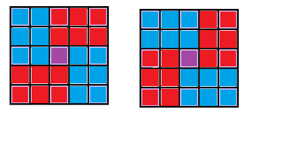
In the drawing, Iahub's possible visited cells are blue, Iahubina's possible visited cells are red and meeting cell is purple. Denote (X, Y) meeting cell.

For first case, Iahub comes from (1, 1) to (X, Y — 1) by going down or right. Next, he goes from (X, Y + 1) to (N, M) by going down or right. Iahubina goes from (M, 1) to (X + 1, Y) by going up or right and then from (X — 1, Y) to (1, M) by going with same directions. In second case, Iahub goes from (1, 1) to (X — 1, Y) and then from (X + 1, Y) to (N, M) and Iahubina goes from (M, 1) to (X, Y — 1) and then from (X, Y + 1) to (1, M).

We can precalculate for dynamic programming matrixes and we're done.

dp1[i][j] = maximal cost of a path going from (1, 1) to (i, j) only down and right.

dp2[i][j] = maximal cost of a path from (i, j) to (1, m) going only up and right.

dp3[i][j] = maximal cost of a path from (m, 1) to (i, j) going only up and right.

dp4[i][j] = maximal cost of a path from (i, j) to (n, m) going only down or right.

And here is my full implementation of recurrences (C++ only):

for (int i = 1; i <= n; ++i)
    for (int j = 1; j <= m; ++j)
        dp1[i][j] = a[i][j] + max(dp1[i - 1][j], dp1[i][j - 1]);
for (int j = m; j >= 1; --j)
    for (int i = 1; i <= n; ++i)
        dp2[i][j] = a[i][j] + max(dp2[i - 1][j], dp2[i][j + 1]);
for (int i = n; i >= 1; --i)
    for (int j = 1; j <= m; ++j)
        dp3[i][j] = a[i][j] + max(dp3[i + 1][j], dp3[i][j - 1]);
for (int i = n; i >= 1; --i)
    for (int j = m; j >= 1; --j)
        dp4[i][j] = a[i][j] + max(dp4[i][j + 1], dp4[i + 1][j]);

Also, pay attention that meeting points can be cells (i, j) with 1 < i < n and 1 < j < m. (why?)

429C - Guess the Tree

The constrain n <= 24 immediately suggest us an exponential solution. 24 numbers seems to be not too big, but also not too small. What if we can reduce it by half? We can do this, by analyzing problem’s restriction more carefully.

The problem states that each internal node has at least two sons. After drawing some trees likes these, one may notice there are a lot of leafs in them. For a tree with this property, number of leafs is at least (n + 1) / 2. We’ll proof this affirmation by mathematical induction. For n = 1, affirmation is true. Now, suppose our tree has n nodes, and the root of it has sons {s1, s2, ..., sk}. Let’s assume subtree of s1 has n1 nodes, subtree of s2 has n2 nodes, ..., subtree of sk has nk nodes. By induction we get that s1 has at least (n1 + 1) / 2 leafs, ..., sk has at least (nk + 1) / 2 leafs. Summing up, we get that our tree has at least (n1 + n2 + ... + nk + k) / 2 leafs. But n1 + n2 + ... + nk = n – 1. So it has at least (n + k – 1) / 2 leafs. But, by hypothesis k >= 2, so our tree has at least (n + 1) / 2 leafs.

For n = 24, there will be at least 13 leafs, so at most 11 internal nodes. It looks much better now for an exponential solution! Before presenting it, we need one more observation. Suppose we sorted c[] array decreasing. Now, the father of node i can be only one of nodes {1, 2, ..., i – 1}. Nodes {i + 1, i + 2, ..., n} will have at most as much nodes as node i, so they can’t be father of i. By doing this observation we can start algorithm: start with node 1 and assign its sons. Then, move to node 2. If it does not have a father, we won’t have one, so current configuration is good. If he has a father (in this case node 1), then tree is connected so far. So we can assign children of node 2. Generally, if a node i does not have a father when it’s processed, it won’t have in future either. If it has, the tree is connected so far, so we add children of i.

Let’s introduce the following dynamic programming. Let dp[node][mask][leafs] = is it possible to create a tree if all nodes {1, 2, ..., node} have already a father, exactly leafs nodes don’t have one and internal nodes corresponding to 1 in bitmask mask also don’t have one? If you never heart about “bitmask” word, this problem is not good for you to start with. I recommend you problem E from round #191, where I explained more how bitmasks work. Back on the problem. If node has 1 in its bit from the mask, then we know for sure the tree can’t be built. Otherwise, let’s assign sons for node. We take all submasks of mask (number obtained by changing some bits from 1 to 0) and make sum of degrees for corresponding nodes. Denote this number as S. These are the internal nodes. How about the leafs? We need to have available L = c[node] – S – 1 leafs. If L is <= than leafs, we can use them. If L < 0, obviously we can’t build the tree. Will remain obviously leafs – L leafs. The new mask will be mask ^ submask. Also, we need to iterate to node + 1. If dp[node+1][mask ^ submask][leafs – L]. One more condition that needs to be considered: node needs to have at least 2 sons. This means L + cnt > 1 (where cnt are number of internal nodes used). When do we stop the dp? When c[nod] = 1. If mask = 0 and leafs = 0, then we can build the tree. Otherwise, we can’t.

Let’s analyze the complexity. There are O(2 ^ (n / 2)) masks, each of them has O(n) leafs, for each O(n) node. This gives O(2 ^ (n / 2) * n ^ 2) states. Apparently, iterating over all submasks gives O(2 ^ (n / 2)) time for each submask, so overall complexity should be O(4 ^ (n / 2) * n ^ 2). But this complexity is over rated. Taking all submasks for all masks takes O(3 ^ (n / 2)) time, instead of O(4 ^ (n / 2)) time. Why? Consider numbers written in base 3: for a mask and a submask we can assign 3 ternary digits to each bit:

0 if bit does not appear in mask

1 if bit appears in mask but not in submask

2 if bit appears in mask and in submask

Obviously, there are O(3 ^ (n / 2)) numbers like this and the two problems are equivalent, so this step takes O(3 ^ (n / 2)) and overall complexity is O(3 ^ (n / 2) * n ^ 2).

429D - Tricky Function

Let’s define S[i] = a[1] + a[2] + ... + a[i]. Then, f(i, j) = (i – j) ^ 2 + (S[i] – S[j]) ^ 2. Trying to minimize this function seems complicated, so we need to manipulate the formula more. We know from the maths that if f(i, j) is minimized, then also f’(i, j) = sqrt ( (i – j) ^ 2 + (S[i] – S[j]) ^ 2) is also minimized. Does this function look familiar to you? Suppose you get two points in 2D plane: one having coordinates (i, S[i]) and the other one having coordinates (j, S[j]). One can see that f’(i, j) is exactly euclidean distance of those points. So, if f’(i, j) is a distance between two points in plane, when is achieved minimal f’(i, j)? For the closest two points in plane (the points which are located at minimal distance). So, having set of points (i, S[i]), we need to compute closest two points from this plane. There is a classical algorithm that does this in O(n * logn).

429E - Points and Segments

The problem asks you to check the property for an infinity of points. Obviously, we can’t do that. However, we can observe that some contiguous ranges on OX axis have the same rx and bx values. Like a sweep line algorithm, a possible change may appear only when a new segment begins or when an old one ends. So let’s consider set of points formed by all li reunited with set of points formed by all ri. Sort the values increasing. Suppose the set looks like {x1, x2, ..., xk}. Then ranges [0, x1) [x1, x2) ... [xk-1, xk) [xk, infinity) are the only ones that need to be considered. If we can take an arbitrary point from each range and the property is respected for all points, then the drawing is good.

We need to color segments. But each segment is a reunion of ranges like the ones from above. When you color a segment, all ranges from it will be colored too. So, after coloring the segments, for each range, |number of times range was colored with blue – number of times range was colored with red| <= 1.

It’s time to think creative. We can see ranges as vertexes of a graph and segments as edges. For example, if a segment is formed by ranges {Xi, Xi+1, ..., Xj-1, Xj} we add an undirected edge from i to j + 1. We need to color the edges. We divide the graph into connected components and apply same logic for each component. Next, by graph I’ll refer to a connected graph.

Let’s assume that our graph has all degrees even. Then, it admits an eulerian cycle. Suppose {x1, x2, ..., xk} is the list of nodes from the cycle, such as x1-x2 x2-x3 ... xk-x1 are the edges of it, in this order. We apply a rule: if xi < xi+1, we color edge between xi and xi+1 in red. Otherwise, we color it in blue. What happens for a node? Whenever a “red” edge crosses it (for example edge 1-5 crosses node 4) a “blue” edge will always exist to cross it again (for example edge 6-2 crosses node 4). This is because of property of euler cycle: suppose we started from a node x and gone in “left”. We need to return to it, but the only way to do it is an edge which goes to “right”. So, when degrees of graph are all even, for every point on OX axis, difference between rx and bx will be always 0.

Let’s solve the general case now. Some nodes have odd degree. But there will always be an even number of nodes with odd degrees. Why? Suppose the property is respected for some edges added so far and now we add a new one. There are two cases:

1/ the edge connects two nodes with odd degree. in this case, the number of nodes with odd degrees decreases by 2, but its parity does not change.

2/ the edge connects one node with odd degree and one node with even degree. Now, degree of “old” odd one becomes even and degree of “old” even one becomes odd. So number of nodes with odd degrees does not change.

So suppose the nodes with odd degrees are X1 X2 ... Xk (k is even). Assume X1 < X2 < ... < Xk. If we add one more edge to each of these nodes, an euler cycle would be possible. However, we can’t “add” edges, because edges are segments from the input. But we can imagine them. Of course, this we’ll create an imbalance between red and blue edges, but let’s see how big it is. What if we add a fictive edge between X1 to X2, between X3 to X4, ..., between X(k – 1) to Xk? In this way, all those nodes will have even degree. So for each Xi (i odd) we add a dummy vertex Yi and some dummy edges from Xi to Yi and from Yi to Xi+1. Now let’s see the effect: if the fictive edges existed, the balance would be 0. But they do not exist, so one of rx or bx will decrease. So now |rx – bx| <= 1, good enough for problem’s restrictions.

Hello everyone!

We invite you to participate in Codeforces Round #245, scheduled for Sunday, 11th May at 7:30 MSK. This is the fourth round I write for Codeforces. After the last round your upvotes helped me get into the Contributors Top 10. Thanks for all your good remarks; I'll try and do my best in order for this round to be at least as good as the previous one.

This round is prepared by my friend Ioan Petcu (author of D1 E) and I (all problems, except D1 E). We've chosen the problems to be as diverse as possible — no two problems will share the same programming technique. As the problems are varied, we hope you'll find at least one problem of your taste. The main character is Iahub, currently the number one ranked contestant in the Romanian selection camps for IOI. After reading the problem statements, you'll see what the life of a very good Romanian competitive programmer is like (just kidding, it's just my evil imagination).

This round wouldn't have been possible without the people that helped me test it: Gerald Agapov (Gerald), Damian Straszak (DamianS), Dan Alexandru (DanAlex) and Vlad Badelita (vladb). As always, we’d like to thank Mike Mirzayanov for creating the Polygon system and Codeforces plaftorm and to Delinur for translating the problems in Russian.

We wish high ratings to everyone and, above all, have fun!

UPD Score Distribution

Division 1: 500 1000 1500 2000 2000

Division 2: 500 1000 1500 2000 2500

I apologize for all technical issues during the round, from the ambiguous problem statements to very easy problem D1 D. In my trial to invent a nice task, I didn't see that straight forward solution for it and I have no excuse for this.

UPD Winners

Division 1:

1. SergeyRogulenko
2. scott_wu
3. vepifanov
4. YuukaKazami
5. ballon

Division 2:

1. clavichord93
2. krmunn481
3. Dgleich
4. PopovkinAndrey
5. roben_76

UPD Editorial

UPD Statistics

384A - Coder

Usually, when you don’t have any idea how to approach a problem, a good try is to take some small examples.

So let’s see how it looks for N = 1, 2, 3, 4 and 5. With C I noted the coder and with * I noted an empty cell.

By now you should note that answer is N ^ 2 / 2 when N is even and (N ^ 2 + 1) / 2 when N is odd. Good. Generally, after you find a possible solution by taking examples, you need to prove it, then you can code it.

In order to proof it, one needs to do following steps:

1/ prove you can always build a solution having N ^ 2 / 2 (or (N ^ 2 + 1) / 2) pieces.

2/ prove that N ^ 2 / 2 (or (N ^ 2 + 1) / 2) is maximal number – no other bigger solution can be obtained.

For proof 1/ imagine you do coloring like in a chess table.

The key observation is that by placing all coders on black squares of table, no two coders will attack. Why? Because a piece placed at a black square can attack only a piece placed at a white square. Again, why? Suppose chess table is 1-based. Then, a square (i, j) is black if and only if i + j is even. A piece placed at (i, j) can attack (i + 1, j), (i – 1, j) (i, j + 1) or (i, j – 1). The sum of those cells is i + j + 1 or i + j – 1. But since i + j is even, i + j + 1 and i + j – 1 are odd, hence white cells.

Depending on parity of N, number of black cells is either N ^ 2 / 2 or (N ^ 2 + 1) / 2. For N even, one can observe that there are equal amount of black and white cells. Total number of cells is N ^ 2, so number of black cells is N ^ 2 / 2. For N odd, number of black cells is number of white cells + 1. We can imaginary add a white cell to the board. Now, number of black cells will be also equal to number of white cells, so answer is (N ^ 2 + 1) / 2.

2/ Two coders attack each other if they are placed at two adjacent cells, one black and other one white. One needs to prove that adding more than number from 1/ will cause this to happen. If you place a coder at a white cell, you won’t be able to place at least one coder at a black cell, so in best case you don’t win anything by doing this. Hence, it’s optimally to place all coders on same color cells. Since cells colored in black are always more or equal to white ones, it’s always optimally to choose black color. But number from 1/ is the number of cells having black color. Adding one more piece will force you to add it to a white color cell. Now, you’ll have a piece placed at a black colored cell and one placed at an adjacent white colored cell, so two coders will attack. Hence, we can’t place more than number from 1/ pieces.

Code: http://pastie.org/8651801

384B - Multitasking

Let’s start by saying when array A[] is sorted:

1/ is sorted in ascending order when i < j and A[i] <= A[j]. It is NOT sorted when i < j and A[i] > A[j].

2/ is sorted in descending order when i > j and A[i] <= A[j]. It is NOT sorted when i > j and A[i] > A[j].

Iahub can choose 2 indices i, j and swap values when A[i] > A[j]. If A[i] <= A[j], he’ll ignore operation. Hence, if he wants to sort all arrays in ascending order, he chooses indices i, j when i < j and perform operation. Otherwise, in all his operations he uses indices i, j such as i > j. A “good” operation is when choosing indices i < j for ascending order sorting and i > j for descending order sorting. By doing only good operations, after an array is sorted, it will stay sorted forever (for a sorted array, all good operations will be ignored).

From here we get our first idea: use any sorting algorithm you know and sort each array individually. When print swaps done by sorting algorithm chosen, print them as good operations. However, sorting each array individually can cause exceeding M * (M — 1) / 2 operations limit. Another possible solution would be, after you did an operation to an array, to update the operation to all arrays (you printed it, so it counts to M * (M — 1) / 2 operations limit; making it to all arrays will help sometimes and in worst case it won’t change anything). However, you need to code it very careful in order to make this algorithm pass the time limit. Doing this in a contest is not the best idea, especially when implementation could be complicated and you have no guarantee it will pass time limit.

So what else can we do? We can think out of box. Instead of sorting specific N arrays, you can sort all possible arrays of length M. Find a sequence of good operations such as, anyhow I’d choose an array of size M, it will get sorted ascending / descending.

I’ll show firstly how to do for ascending sorting. At position 1 it needs to be minimal element. Can we bring minimal element there using good operations? Yes. Just do “1 2” “1 3” “1 4” ... “1 M”. It basically compares element from position 1 to any other element from array. When other element has smaller value, swap is done. After comparing with all M elements, minimal value will be at position 1. By now on I’ll ignore position 1 and move to position 2. Suppose array starts from position 2. It also needs minimal value from array, except value from position 1 (which is no longer in array). Hence doing “2 3” “2 4” “2 5” ... “2 M” is enough, by similar reasons. For a position i, I need minimal value from array, except positions 1, 2, ..., i – 1. I simply do “i i+1” “i i+2” ... “i M-1” “i M”. By arriving at position i, array will be sorted ascending. The algorithm is simply:

for (int i = 1; i < M; ++i)

for (int j = i + 1; j <= M; ++j)

cout << i << “ “ << j << “\n”;

This algorithm does exactly M * (M — 1) / 2 moves.

Can you find out how to sort array in descending order? Try to think yourself, then if you don’t get it read next. At first position of a descending array it needs to be maximal value. Similarly to ascending order, we can do “2 1” “3 1” “4 1” ... “M 1”. When I’m at a position i and I compare its value to value from position 1, doing operation “i 1” checks if A[i] > A[1]. If so, it swaps A[i] and A[1], so position 1 will contain now the maximum value so far. Similarly to logic from ascending order, when I’m at position i, I need maximum value from array except positions 1, 2, ..., i – 1, so I do “i+1 i” “i+2 i” ... “M i”. Algorithm is:

for (int i = 1; i < M; ++i)

for (int j = i + 1; j <= M; ++j)

cout << j << “ “ << i << “\n”;

Obviously, this does as well M * (M — 1) / 2 operations worst case. All algorithm is about 10 lines of code, much better than other solution, which requires two manually sorts and also has a chance to exceed TL.

Code: http://pastie.org/8651809

384C - Milking cows

A good strategy to approach this problem is to think how optimal ordering should look like. For this, let’s calculate for each 2 different cows i and j if cow i needs to be milked before or after cow j. As we’ll show, having this information will be enough to build optimal ordering. It is enough to consider only cases when i < j, case when i > j is exactly the opposite of case i < j. For formality, I’ll call the optimal ordering permutation and lost milk the cost of permutation.

So, for an optimal permutation P let’s take 2 numbers i < j and see in which cases i should appear before j in permutation (i is before j if P[pos1] = i, P[pos2] = j and pos1 < pos2; otherwise we’ll call i is after j). We have 4 possible cases:

1/ A[i] = 0 and A[j] = 0

If we put i before j, no additional cost will be added. Since j is in right of i and i only adds cost when it finds elements in left of i, j won’t be affected when processing i. When processing j, i will be already deleted so it won’t affect the cost either. Hence, we can put i before j and no cost will be added.

2/ A[i] = 0 and A[j] = 1

Here, i and j can appear in arbitrary order in permutation (i can be before or after j). No matter how we choose them, they won’t affect each other and cost will remain the same.

3/ A[i] = 1 and A[j] = 0

As well, here i and j can appear in arbitrary order. If we choose i first, j will be in right of it, so cost of permutation will increase by one. If we choose j first, i will be in left of it so cost of permutation will increase as well. No matter what we do, in this case cost of permutation increases by 1.

4/ A[i] = 1 and A[j] = 1

Here, i needs to be after j. This adds 0 cost. Taking i before j will add 1 cost to permutation (since j is in right of i).

Those 4 cases show us how a minimal cost permutation should look. In a permutation like this, only case 3/ contributes to final cost, so we need to count number of indices i, j such as i < j and A[i] = 1 and A[j] = 0 (*). If we show a permutation following all rules exists, task reduces to (*).

By cases 2/ and 3/ it follows that in an optimal permutation, it only matters order of elements having same value in A[]. We can put firstly all elements having value 0 in A[], then all elements having value 1 in A[]. We can order elements having value 0 by case 1/ and elements having value 1 by case 4/. More exactly, suppose i1 < i2 < ... < im and (A[i1] = A[i2] = ... = A[im] = 0) and j1 > j2 > ... > jn (A[j1] = A[j2] = ... = A[jn] = 1). Then, a permutation following all rules is {i1, i2, ..., im, j1, j2, ..., jn}. This permutation can always be built.

Hence, task reduces to (*): count number of indices i, j such as i < j and A[i] = 1 and A[j] = 0. We can achieve easily an O(N) algorithm to do this. Let’s build an array cnt[j] = number of 0s in range {j, j + 1, ..., N} from array A. We can easily implement it by going backwards from N to 1. The result is sum of cnt[i], when A[i] = 1.

Code: http://pastie.org/8651813

384D - Volcanoes

Our first observation is that if there is a path from (1, 1) to (N, N), then the length of path is 2 * N – 2. Since all paths have length 2 * N – 2, it follows that if there is at least one path, the answer is 2 * N – 2 and if there isn’t, the answer is -1. How to prove it? Every path from (1, 1) to (N, N) has exactly N – 1 down directions and exactly N – 1 right directions. So, total length for each path is N – 1 + N – 1 = 2 * N – 2.

So we reduced our problem to determine if there is at least one path from (1, 1) to (N, N). This is the challenging part of this task, considering that N <= 10 ^ 9. How would you do it for a decently small N, let’s say N <= 10^3 . One possible approach would be, for each row, keep a set of reachable columns. We could easily solve this one by doing this: if (i, j) denotes element from ith row and jth column, then (i, j) is (is not) reachable if:

if (i, j) contains a volcano, then (i, j) is not reachable. Otherwise, if at least one of (i – 1, j) and (i, j – 1) is reachable, then (i, j) is reachable. Otherwise, (i, j) is not reachable.

What’s the main problem of this approach? It needs to keep track of 10^9 lines and in worst case, each of those lines can have 10^9 reachable elements. So, worst case we need 10^9 * 10^9 = 10^18 operations and memory.

Can we optimize it? We can note for beginning that we don’t need to keep track of 10^9 lines, only m lines are really necessarily. We need only lines containing at least one obstacle (in worst case when each line contains only one obstacle, we need m lines). How to solve it this way? Suppose line number x contains some obstacles and lines x + 1, x + 2, x + 3 do not contain any obstacle. Suppose we calculated set S = {y | cell (x, y) is reachable}. How would look S1, S2, S3 corresponding to lines x + 1, x + 2, x + 3? For S1, we can reach cell (x + 1, ymin), where ymin is minimal value from set S. Then, we can also reach {ymin + 1, ymin + 2, ..., N}, by moving right from (x + 1, ymin). So S1 = {ymin, ymin + 1, ..., N}. How do S2 and S3 look? It’s easy to see that they’ll be as well {ymin, ymin + 1, ..., N}. So we get following optimization: suppose set of lines containing at least one obstacle is {L1, L2, ..., Lk}. We need to run algorithm only for lines L1, L1 + 1, L2, L2 + 1, L3, L3 + 1, ..., Lk, Lk + 1.

It looks like we didn’t make anything with this optimization. Even if we calculate for m lines, each line can still have 10^9 reachable positions. So worst case we perform 10^14 operations. We need something better for managing information from a line. You can note that for a given line y, there are a lot of positions having consecutive values. There are a lot of positions (x, y) and (x, y + 1) both reachable. This should give us following idea: what if instead of keeping reachable positions, we keep reachable ranges? That is, for each line x we keep a set of ranges S = {(a, b) | all cells (x, k) with a <= k <= b are reachable}.

How many ranges can it be for a line? If the line contains m obstacles, there are m + 1 ranges. Suppose for line x all cells are reachable, but for line x + 1 cells (x + 1, 3) (x + 1, 5) (x + 1, N – 1) are blocked. Then, the ranges of reachable cells are [1, 2] [4, 4], [6, N – 2] and [N, N]. By now, we get worst case m lines and worst case each line having m elements, so in worst case we’d have to handle m * m = 10 ^ 10 events. This may still look too much, but happily this bound is over estimated. If a line has o obstacles, there can be at most o + 1 ranges. If lines L1, L2, ..., Lk have {o1, o2, ..., ok} obstacles, there’ll be at most o1 + o2 + ... + ok + k ranges. But o1 + o2 + ... + ok = m and also k is at most m (proved above why we’re interested in at most m lines), so in worst case we get m + m = 2 * m ranges. Yaay, finally a decent number of states for this problem :)

So, we iterate each line we’re interested in. Let’s find set of ranges for this line, thinking that all cells from line above are reachable. This is easy to do. After we get our ranges like all cells from above can be visited, let’s think how having obstacles above can influence current ranges. After adding ranges from above, current ranges can’t increase (obviously), they can only decrease, remain the same or some of them can become empty. So, let’s take each range [a, b] from current line and see how it will transform after adding ranges from previous line.

Given range [a, b], it can transform only in [a’ , b] with a’ >= a. If a’ > b, then obviously range is empty. Why second number of range keeps constant? Let a’ smallest reachable column from current line which is in range [a, b]. It’s enough to check a’ >= a, as if a’ > b, range will be empty. It’s obviously why we need to keep a’ smallest value possible >= a: we’re interested to keep range as big as possible and as less as we cut from left, as big it is. Once we’ve found a’ in range [a, b] (or a’ > b if range is empty) all cells {a’ + 1, a’ + 2, ..., b} are reachable as well by going right from a’, so if interval is not empty, then second number defining it remains b.

Next question is how to find a’ fast enough. In order a point a’ to be reachable on current range, it also needs to exist a range on previous line containing it. If the range from previous line is [pa, pb] then a’ needs to follow 3 conditions:

a’ minimal such as

pa <= a’ <= pb

a’ >= a

What if instead of finding a’ we find [pa, pb]? Then a’ is max(pa, a). In order a’ to be as small as possible, since a is constant, pa needs to be as small as possible. So we reduced it to:

pa minimal pb >= a’ >= a <=> pb >= a

Intervals from previous line are disjoint, no 2 intervals cross each other. It means that if pb is minimal, than pa is minimal too (if we increase pb, then pa will increase too, so it won’t be minimal). Hence, you need to find an interval [pa, pb] such as pb is minimal and pb >= a. Then, a’ is max(a, pa). This is easy to do if we sort all intervals from previous line increasing by second value (pb), then we binary search for value a.

Finally, after running algorithm for all lines, last range from last line has second number N (assuming ranges are sorted increasing by second value), then there exist a path, otherwise there does not exist. This algorithm should run O(m * logm) worst case, good enough to pass.

Code: http://pastie.org/8651817

384E - Propagating tree

This is kind of task that needs to be break into smaller subproblems that you can solve independently, then put them together and get solution.

Let’s define level of a node the number of edges in the path from root to the node. Root (node 1) is at level 0, sons of root are at level 1, sons of sons of root are at level 2 and so on.

Now suppose you want to do an operation of type 1 to a node x. What nodes from subtree of x will be added +val (a positive value)? Obviously, x will be first, being located at level L. Sons of x, located at level L + 1 will be added –val. Sons of sons, located at level L + 2, will be added value +val again. So, nodes from subtree of x located at levels L, L + 2, L + 4, ... will be added a +val, and nodes located at levels L + 1, L + 3, L + 5 will be added a –val. Let’s take those values of L modulo 2. All nodes having remainder L modulo 2 will be added a +val, and nodes having reminder (L + 1) modulo 2 will be added –val. In other words, for a fixed x, at a level L, let y a node from subtree of x, at level L2. If L and L2 have same parity, +val will be added to y. Otherwise, -val will be added to y.

From here we have the idea to split nodes of tree in 2 sets – those being located at even level and those being located at odd level. What still makes the problem hard to solve? The fact that we have a tree. If nodes from a subtree would be a contiguous sequence instead of some nodes from a tree, problem would be simpler: the problem would reduce to add / subtract values to all elements of a subarray and query about a current value of an element of array. So, how can we transform tree to an array, such as for a node x, all nodes from subtree of x to be a subarray of array?

The answer is yes. We can do this by properties of DFS search. Before reading on, make sure that you know what is discovery time and finish time in a DFS search. Let’s build 3 arrays now – discover[], representing nodes in order of their discover times (a node is as before in discover as it has a small discover time), begin[] = for a node, in which time it was discovered and end[] = what’s last time of a discovered node before this node finishes. For a subtree of x, all nodes in the subtree are nodes in discover from position begin[x] to end[x].

Example: suppose you have tree 1-5; 1-6; 6-7; 6-4; 4-2; 4-3

Discover is {1, 5, 6, 7, 4, 2, 3}.

begin is {1, 6, 7, 5, 2, 3, 4}.

end is {7, 6, 7, 7, 2, 7, 4}.

What’s subtree of node 6? elements of discover from position begin[6] to end[6]. In this case, from 3 to 7, so elements {6, 7, 4, 2, 3}. You can see it’s correct and take more examples if you want :)

Now, we reduced problem to: you’re given an array A. you can perform 2 operations:

1/ increase all elements from a range [x, y] to a value val (val can be negative, to treat subtractions)

2/ what’s current value of an element from position pos.

Those who solved “Iahub and Xors” from my last round, CF 198, should probably say they saw something similar before. If you didn’t solve problem before, I encourage you to do it after you solve this one, it uses a similar idea to what will follow now. Also, if you don’t know Fenwick trees, please read them before moving on. An alternative would be for this task using segment trees with lazy update, but I see this one more complicated than needed.

I’ll use now a not so common approach when dealing with data structures. Instead of keeping in a node the result, like you usually do, I’ll keep just an auxiliary information. So what algorithm proposed does:

Let A an array, initially with all elements 0.

When you need to update range [x, y] with value val, you simply do A[x] += val and A[y + 1] -= val.

When you need to answer a query about position pos, you output A[1] + A[2] + ... + A[pos].

Implemented brute force, you get O(1) per update and O(N) per query. However, these both are operations supported by a Fenwick tree, so you can get O(logN) per operation.

It may not be very clear why this algorithm works. Let’s take a closer look: an update needs to add value val only to range [x, y]. When you query a position pos, let’s see if algorithm handles it correctly:

1/ pos < x. In this case, result must not be affected by my update. Since pos < x and I only updated 2 values with indices >= x, when doing A[1] + A[2] + ... + A[pos] it won’t matter at all I did that update – at least not for this query.

2/ x <= pos <= y. Here, for a pos, I need to add value val only once. We add it only at A[x] – in this way it will be counted once, and it will be considered for each elements from range [x, y] (since an element at position p from range [x, y] has p >= x, in A[1] + A[2] + ... + A[p] I’ll have to consider A[x]).

3/ pos > y. Here I don’t have to consider the query. But it would be considered when processing A[x]. But if I add to A[y + 1] value –val I’ll just cancel the value previously added.

Code (actually we use just one Fenwick tree instead of 2, can you think why it works? :) ) : http://pastie.org/8651824

383D - Antimatter

Author's solution

The problem is: given an array, iterate all possible subarrays (all possible elements such as their indexes are consecutive). Now, for a fixed subarray we need to know in how many ways we can color its elements in black and white, such as sum of black elements is equal to sum of white elements. The result is sum of this number, for each subarray.

Let’s solve an easier problem first. This won’t immediately solve the harder version, but it will be useful later. Suppose you’ve fixed a subarray. In how many ways can you color it with black and white? Suppose subarray has N elements and sum of them is M. Also, suppose for a coloring, sum of blacks is sB and sum of whites is sW. For coloring to be valid, sB = sW. But we also know that sB + sW = M (because each element is colored by exactly one color). We get that 2 * sB = M, so sB = M / 2. The problem is now: in how many ways can we color elements in black such as sum of blacks is M / 2 (after we fix a black coloring, we color with white non colored elements; sum of white colored elements is also M / 2). This is a well known problem: Knapsack problem. Let ways[i][j] = in how many ways one can obtain sum j from first i elements. When adding (i + 1) object, after ways[i] is calculated, for a fixed sum j we can do 2 things: add (i + 1) object to sum j or skip it. Depending of what we chosen, we add value ways[i][j] to ways[i + 1][j + value[i + 1]] or to ways[i + 1][j]. The result is in ways[N][M / 2]. This works in O(N * M) time.

An immediate solution can be obtained now: take all subarrays and apply above approach. This leads to an O(N ^ 2 * M ^ 2) solution, which is too much. One can reduce complexity to O(N ^ 2* M) by noting that processing subarray [i, j] can be done with already calculated values for subarray [i, j – 1]. Hence, instead of adding N elements, it’s enough to add 1 element to already calculated values (element from position j). Sadly, O(N ^ 2 * M) is still too slow, so we need to find something better. The solution presented below will look forced if you didn’t solve some problems with this technique before. It’s hard to come with an approach without practicing this kind of tasks. But don’t worry, as much as you practice them, as easily you’ll solve those problems.

We’ll solve task by divide and conquer. Complexity of this solution is O(N * M * logN). Let f(left, right) a function that counts number of colorings for each subarray [i, j], such as subarray [i, j] is included in subarray [left, right] (left <= i <= j <= right). Answer is in f(1, N). The trick is to define a value med = (left + right) / 2 (very frequent trick in divide and conquer problems, called usually a median). We can next classify [i, j] subarrays in 3 types:

1/ i <= med j <= med

2/ i > med j > med

3/ i <= med j > med

We can solve 1/ and 2/ by calling f(left, med) and f(med + 1, right). The remained problem is when i <= med and j > med. If we solve 3/ in O((right – left) * M) time, this will be enough to overall achieve O(N * M * logN) (for this moment trust me, you’ll see later why it’s so :) ).

Let’s denote by i1 last i1 elements from subarray [left, med]. Also, let’s note by i2 first i2 elements from subarray [med + 1, right]. For example, let left = 1 and right = 5, with array {1, 2, 3, 4, 5}. med is 3 and for i1 = 2 and i2 = 1, “left” subarray is {2, 3} and “right” subarray is {4}. By iterating i1 from 1 to med – left + 1 and i2 from 1 to right – med and then unite subarrays i1 and i2, we obtain all subarrays described in 3/ . Let’s denote by j1 sum of a possible black coloring of i1. Similarly, j2 is sum of a possible black coloring of i2.

Suppose we fixed i1, i2, j1 and j2. When it’s the coloring valid? Let S sum of united subarrays i1 and i2 (S = value[med – i1 + 1] + value[med – i1 + 2] + ... + value[med] + value[med + 1] + ... + value[med + i2 – 1] + value[med + i2]). Now it’s time to use what I explained at the beginning of solution. The coloring is good only when j1 + j2 = S / 2. We can rewrite the relation as 2 * (j1 + j2) = sum_of_elements_from_i1 + sum_of_elements_from_i2. We can rewrite it even more:

2 * j1 + 2 * j2 — sum_of_elements_from_i1 — sum_of_elements_from_i2 = 0

2 * j1 – sum_of_elements_from_i1 = sum_of_elements_from_i2 – 2 * j2 = combination_value

This relation is the key of solving problem. You can see now that relation is independent in “left” and “right” side. We calculate left[i1][j1] and right[i2][j2] = in how many ways can I obtain sum of blacks j1 (j2) from first i1 (i2) from left (right) side. Let’s calculate also count[value] = in how many ways can I obtain combination_value equal to value in the right side. For some fixed (i2, j2) I add to count[sum_of_elements_from_i2 – 2 * j2] value right[i2][j2]. In this way count[] is calculated correctly and completely. Now, let’s fix a sum (i1, j1) in the left side. We’re interested how many good colorings are such as there exist a coloring of j1 in i1 elements (the endpoint of “left” is fixed to be i1 and I need to calculate endpoints i2 for right, then to make colorings of i2). A coloring is good if combination_value of (i1, j1) and (i2, j2) is equal. Hence, I need to know in how many ways I can color i1 elements to obtain sum j1 and also I need to know in how many ways I can color elements from right to obtain same combination_value as it’s in the left. It’s not hard to see that answer for a fixed (i1, j1) is left[i1][j1] * count[2 * j1 – sum_of_elements_from_i1]. This takes O((right – left) * M) time.

The only thing remained in the problem is to see why complexity is O(N * M * logN). We can assume N is a power of 2 (it not, let’s round N to smallest power of 2 bigger than N; complexity for N is at least as good as complexity for this number). Draw a binary complete tree with N nodes. Each node corresponds to an appeal of f(). For a level, exactly O(N * M) operations are performed. To see why:

For level 1, there’ll be 1 node performing N * M operations.

For level 2, there’ll be 2 nodes performing (N / 2) * M operations. Summing up we get O(N * M).

For level 3, there’ll be 4 nodes performing (N / 4) * M operations. Summing up we get O(N *M) as well.

and so on.

So for each level we perform O(N * M) operations. A binary complete tree has maximum O(logN) levels, so overall complexity is O(N * M * logN).

Code: http://pastie.org/8651826

Solution fount by contestants

This was totally unexpected to us :) Good job finding it, you guys are really smart.

We observe that x units of antimatter is the same thing as -x units of matter. Then we can consider that an element produces either x or -x units of matter. A valid substring is one that can have the sum of the elements 0. The problem is reduced to finding how many different substrings can we have with sum 0 (a substring is different than another one if it has different indices, or if at least one element produces matter in one and antimatter in the other).

This problem can be solved with dynamic programming. We will hold D[i][j] = the number of substrings that end in element i, and have sum j. It's easy to see that D[i + 1][j] = D[i][j — x] + D[i][j + x], where x is the value of the current element (we can put either -x or x). After we finish computing all the values for current i, we add to the solution D[i][0] (how many valid substrings do we have). After that, we add 1 to D[i][0], meaning that there is an empty substring starting at position i (however, we don't need to add it to the answer).

For a code, check passing submissions during contest.

383E - Vowels

Author's solution

Let's iterate over all possible vowel sets. For a given set {x1, x2, ..., xk} we're interested in number of correct words from dictionary. After a precalculation, we can do it in O(k).

Suppose our current vowel set is {x1, x2, ..., xk}. How many words are covered by the current vowels? By definition, we say a word is covered by a set of vowels if at least one of 3 letters of word is in vowel set. We can calculate this number using principle of inclusion and exclusion. We’ll denote by |v1, v2, v3, ...| = number of words containing ALL of vowels v1, v2, v3, ... . Using principle of inclusion and exclusion we get:

number_of_words_covered = |x1| + |x2| + .. + |xk| — |x1, x2| — |x1, x3| — .... + |x1, x2, x3| + |x1, x2, x4| + .... + |xk-2, xk-1, xk|. This formula is simply a reformulation of principle of inclusion and exclusion. You can easily observe that |v1, v2, ..., vk| makes sense only when k is at most 3, as no word from input can contain 4 or more letters (and hence can’t contain 4 or more vowels).

Example:

Suppose words are abc, abd and bcd.

|a| = 2 (first 2 words both contain character a).

|a, b| = 2 (as well, first 2 words contain characters a and b).

|b| = 3 (all 3 words contain character b).

|a, b, d| = 1 (only second word contains all 3 characters).

Also, note how principle of inclusion and exclusion works. number of words covered for vowels {a, b} is |a| + |b| — |a, b| = 2 + 3 – 2. Indeed, answer is 3.

We divide our problem in 3 subproblems. First one, for a vowel set, compute sum of |a|, where a is a letter from subset. Second, compute sum of |a, b|, where both a and b are letters from set. Third, compute sum of |a, b, c|, where a, b, c are letters from set. As stated, the answer is number_from_1st_step + number_from_3rd_step – number_from_2nd_step. If you followed me, you’ll see that we want to compute results for each subproblem in O(queryLetters).

First subproblem can be solved trivially in O(queryLetters). Let array single[], with following meaning: single[c] is how many words contain character c. It can be trivially precomputed in O(24 * N). Note that if a word contains twice/third times a character c, it needs to be counted only one (e.g. word aba will add only 1 to single[a]). For compute result of this subproblem for a given set of vowels, I’ll take all letters from set. If letter belongs to set, I add to result single[letter]. This step can be also be solved in O(1), but there’s no need, since other subproblems allow only an O(queryLetters) solution.

For second and third subproblems it’s a little more difficult. I’ll present here how to solve second subproblem and some hints for third one (if you understand second, with hints you should be able to solve third one by your own).

Similarly to first step, I’ll define a matrix double[c1][c2] = how many words contain both characters c1 and c2. A trivially solution would be, for a given vowel set, take all combinations of letters c1 and c2 that belong to set and add to result value double[c1][c2]. However, this solves each query in O(queryLetters^2), which is too slow.

Note, if we’d have 12 letters, instead of 24, this approach would be fast enough. From here it comes a pretty classical idea in exponential optimization: meet in the middle attack. We split those 24 letters in 2 groups: first 12 letters and last 12 letters. The answer for a subset is sum of double[c1][c2] (when c1 and c2 belong to current vowel set) when

1/ c1 and c2 belong to first 12 letters

2/ c1 and c2 belong to last 12 letters

3/ c1 belongs to first 12 letters and c2 belongs to last 12 letters

1/ and 2/ can be immediately precalculated as stated above, in O(2 ^ 12 * 12 ^ 2). We’ll remember results for each half using bitmasks arrays. Let Half1[mask] = sum over double[c1][c2], when c1 and c2 are in first 12 letters and correspond to 1 bits of mask. Half2[mask] is defined similarly, but for last 12 letters (e.g. subset {a, c, d} corresponds to bitmask 2^0 + 2^2 + 2^3 = 13 in first half and subset {m, n, p} corresponds to bitmask 2^0 + 2^1 + 2^3 = 11 for second half). Now, for a given subset, one can answer first 2 parts in O(queryCount) worst case (read input for a query and convert it to bitmasks).

How to answer 3? With another precalculation, of course. We know c1 letter needs to be in first 12 letters and c2 needs to be in last 12 letters. The precalculation we do here is: mixed_half[mask][i] = sum over |c1, c2|, when c1 belongs to first half and is a 1 bit of mask and c2 is i-th character of second half. Hence, for a query, we can fix character from second half (c2, by iteration of query letters from second half) and know sums of |c1, c2| between it and all available characters from first half after we do this precalculation. Also, precalculation is done trivially in O(2 ^ 12 * 12^2): fix mask, fix i and then iterate over 1 bits from mask and add double[c1][c2].

Third subproblem is left, but it can be done similarly to second one. Instead of double[c1][c2], we’ll have triple[c1][c2][c3] = how many words contain all 3 characters c1, c2 and c3? We also do meet in the middle here, divide those 24 letters into 2 sets of 12 letters. We have 4 cases:

1/ c1, c2, c3 belong to first half

2/ c1, c2, c3 belong to second half

3/ c1, c2 belong to first half and c3 to second half

4/ c1 belongs to first half and c2, c3 to second half

1/ and 2/ are done brute force, like in second subproblem (the only difference is we choose 3 characters instead of 2, having complexity O(2 ^ 12 * 12 ^ 3)). For 3/ and 4/ we also precompute 2 matrixes:

mixed_two_one[mask][i] = c1 and c2 belong to mask from first half and c3 is i-th character from second half

and

mixed_one_two[mask][i] = c1 is i-th character from first half and c2, c3 belong to mask from second half.

Those can also be calculated in O(2 ^ 12 * 12^3).

So precalculation part is O(2 ^ 12 * 12 ^ 3) = 7077888 operations.

For calculate answering queries complexity, take all numbers from 0 to 2^24 — 1 and sum their bit count. This is a well known problem, the sum is 0 * C(24, 0) + 1 * C(24, 1) + ... + 24 * C(24, 24) = 201326592. In total we get 208404480 operations. C++ source makes them in 2 seconds.

Code: http://pastie.org/8651829

Solution fount by contestants

Like in D1 D task, official solution was over complicated. This solution is more simple to understand, code and it's more elegant. If someone wants to complicate his life, (s)he can code also official solution :)

Let's start by assigning a bitmask to each word in following way: ith bit is 1 if and only if letter ('a' + i) appears in the current word. For example, for word acd, its bitmask is 2^0 + 2^2 + 2 ^ 3 = 13 and for word aab its bitmask is 2^0 + 2^1 = 3. After reading the words from dictionary, we store a matrix cnt[mask] = how many words from dictionary correspond to mask?

We iterate bitmasks from 0 to 2^24 — 1, this time corresponding to each possible question of Iahubina. Let's focus on a bitmask X. We need to get sum of cnt[mask], when mask and X share at least one common bit having value 1 (formally (X AND mask) > 0). In order to do this, we need a reduction which may be not so obvious.

What if instead of counting all words containing at least one of vowels {w1, w2, ..., wk} we count all words which don't contain ANY of vowels {w1, w2, ..., wk}? Suppose this number is ret. Then, all words containing at least one of vowels is N — ret. From all words, we erase those words which do not contain any vowels from set {w1, w2, ..., wk} (and which obviously are wrong words). Obviously, it's left only words containing at least one vowel, so good words. Now, for a word not to contain any of vowels {w1, w2, ..., wk} it needs to contains ONLY vowels from set {"a", "b", "c", ..., "x"} \ {w1, w2, ..., wk} (set of allowed letters from which we erased vowels w1, w2, ..., wk}.

And this is reduction we needed. For a bitmask X we need to calculate sum of cnt[mask], where mask is a subset of X (we can set some bits from X from 1 to 0 in order to obtain mask). For a mask, let's keep this sum in res[mask]. We can calculate res array using divide and conquer.

Let's make a function solve(left, right), which completes array res in the way described above, if we consider only elements cnt[k] with left <= k < right (for simplicity, I'll consider elements which do not lie in this range to be equal to 0). Now we need to solve for a range [left, right]. Let's have in res1[] = solve(left, med) and in res2[] = solve(med, right), where med = (left + right) / 2. We need to put together res1[] and res2[] in order to obtain res[].

for (int i = left; i < med; ++i) res[i] = res1[i];

Numbers in [left, med] have most significant bit equal to 0. We can only keep it 0 and add what we calculated before. We can't add any element from res2[], because those elements have most significant bit equal to 1 and we're not allowed to change bit 0 into bit 1.

for (int i = med; i < right; ++i) res[i] = res1[i — med] + res2[i];

Here, most significant bit is 1. Adding res1[] corresponds to changing bit from 1 to 0, adding res2[] corresponds to leaving bit 1.

Of course, we need to threat the base case here, too. When left + 1 = right, res[left] = cnt[left]. We can keep only one array res[] instead of 3, I explained it this way only for simplicity. Also, there is no need for keeping separate arrays for res[] and cnt[], one can solve all task with only one array. In order to get res[], we simply call solve(0, 2^24).

Complexity of solution is O(2 ^ 24 * 24). I leave the proof homework, it's almost identical to complexity proof of D1 D "Author solution" (that with building a binary tree).

For a reference solution, check Endagorion's AC source during contest.

Hello everyone!

We invite you to participate at Codeforces Round #225, scheduled Monday, 20th January at 7:30 PM MSK. This is the third round I coauthor, along with Codeforces Round 198 (Div. 1) (and of course Div. 2 version of contest) and Codeforces Round 191 (Div. 2).

If you recall my old rounds, you'll see that main character is Iahub. The other writer of this round is... Iahub... the real person corresponding to "Iahub" character. Let me introduce you to Rares Buhai (rares.buhai). He's the author of Div. 2 C / Div. 1 A, Div. 1 D and Div. 1 E. You can expect those problems to be interesting, coming from a 2 times IOI gold medalist (being allowed to participate 2 more times). All other problems are created by me. I like them, but I wouldn't be objective if I said that they're interesting. Let's see if someone will think so after the contest :)

Like last time, I'll give you a little spoiler about the tasks. We tried to make the problem set as varied as possible. In order to get a good rank, one needs to be good at "ad hoc" problems as well as have good algorithmic knowledge.

As always, thanks to MikeMirzayanov for Codeforces platform, to Delinur for translating tasks, to Gerald for helping us prepare the round and to DamianS and ll931110 for testing it.

We wish everyone high rating and to have fun!

UPD Score distribution:

Division 1: 500 — 1500 — 1500 — 2000 — 2500

Division 2: 500 — 1000 — 1500 — 2500 — 2500

UPD Contest is over! Thanks for everyone who participated! I need to say we're impressed of your creative and totally unexpected solutions for Division 1 D.

Div. 1 winners:

1. yeputons
2. Arcueid
3. Dmitry_Egorov
4. ACMonster
5. scott_wu

Div. 2 winners:

1. Sick_coder
2. akaring
3. c0d3junki3
4. raihatneloy
5. sky0917

UPD Editorial

340A - The Wall

You are given a range [A, B]. You're asked to compute fast how many numbers in the range are divisible by both x and y. I'll present here an O(log(max(x, y)) solution. We made tests low so other not optimal solutions to pass as well. The solution refers to the original problem, where x, y ≤ 10⁹.

Firstly, we can simplify the problem. Suppose we can calculate how many numbers are divisible in range [1, X] by both x and y. Can this solve our task? The answer is yes. All numbers in range [1, B] divisible by both numbers should be counted, except the numbers lower than A (1, 2, ..., A — 1). But, as you can see, numbers lower than A divisible by both numbers are actually numbers from range [1, A — 1]. So the answer of our task is f(B) — f(A — 1), where f(X) is how many numbers from 1, 2, ..., X are divisible by both x and y.

For calculate in O(log(max(x, y)) the f(X) we need some math. If you don't know about it, please read firstly about least common multiple. Now, what will be the lowest number divisible by both x and y. The answer is least common multiple of x and y. Let's note it by M. The sequence of the numbers divisible by both x and y is M, 2 * M, 3 * M and so on. As a proof, suppose a number z is divisible by both x and y, but it is not in the above sequence. If a number is divisible by both x and y, it will be divisible by M also. If a number is divisible by M, it will be in the above sequence. Hence, the only way a number to be divisible by both x and y is to be in sequence M, 2 * M, 3 * M, ...

The f(X) calculation reduces to finding the number of numbers from sequence M, 2 * M, 3 * M, ... lower or equal than X. It's obvious that if a number h * M is greater than X, so will be (h + 1) * M, (h + 2) * M and so on. We actually need to find the greatest integer number h such as h * M ≤ X. The numbers we're looking for will be 1 * M, 2 * M, ..., h * M (so their count will be h). The number h is actually [X / M], where [number] denotes the integer part of [number]. Take some examples on paper, you'll see why it's true.

The only thing not discussed is how to calculate the number M given 2 number x and y. You can use this formula M = x * y / gcd(x, y). For calculate gcd(x, y) you can use Euclid's algorithm. Its complexity is O(log(max(x, y)), so this is the running time for the entire algorithm.

Official solution: 4383403

340B - Maximal Area Quadrilateral

I want to apologize for not estimating the real difficulty of this task. It turns out that it was more complicated than we thought it might be. Let's start explanation.

Before reading this, you need to know what is signed area of a triangle (also called cross product or ccw function). Without it, this explanation will make no sense.

The first thing we note is that a quadrilateral self intersecting won't have maximum area. I'll show you this by an image made by my "talents" in Paint :) As you can see, if a quadrilateral self intersects, it can be transformed into one with greater area.

Each quadrilateral has 2 diagonals: connecting 1st and 3rd point and connecting 2nd and 4th point. A diagonal divides a plane into 2 subplanes. Suppose diagonal is AB. A point X can be in one of those two subplanes: that making cross product positive and that making cross product negative. A point is in "positive" subplane if ccw(X, A, B) > 0 and in "negative" subplane ccw(X, A, B) < 0. Note that according to the constraints of the task, ccw(X, A, B) will never be 0.

Let's make now the key observation of the task. We have a quadrilateral. Suppose AB is one of diagonals and C and D the other points from quadrilateral different by A and B. If the current quadrilateral could have maximal area, then one of points from C and D needs to be in "positive subplane" of AB and the other one in "negative subplane". What would happen if C and D will be in the same subplane of AB? The quadrilateral will self intersect. If it will self intersect, it won't have maximal area. "A picture is worth a thousand words" — this couldn't fit better in this case :) Note that the quadrilateral from the below image is A-C-B-D-A.

Out task reduces to fix a diagonal (this taking O(N ^ 2) time) and then choose one point from the positive and the negative subplane of the diagonal. I'll say here how to choose the point from the positive subplane. That from negative subplane can be chosen identically. The diagonal and 3rd point chosen form a triangle. As we want quadrilateral to have maximal area, we need to choose 3rd point such as triangle makes the maximal area. As the positive and negative subplanes are disjoint, the choosing 3rd point from each of them can be made independently. Hence we get O(N ^ 3) complexity. A tricky case is when you choose a diagonal but one of the subplanes is empty. In this case you have to disregard the diagonal and move to the next one.

Official solution: 4383413

340C - Tourist Problem

Despite this is a math task, the only math formula we'll use is that number of permutations with n elements is n!. From this one, we can deduce the whole task.

The average formula is sum_of_all_routes / number_of_routes. As each route is a permutation with n elements, number_of_routes is n!. Next suppose you have a permutation of a: p1, p2, …, pn. The sum for it will be p1 + |p2 – p1| + … + |pn – pn-1|. The sum of routes will be the sum for each possible permutation.

We can calculate sum_of_all routes in two steps: first time we calculate sums like “p1” and then we calculate sums like “|p2 – p1| + … + |pn – pn-1|” for every existing permutation.

First step Each element of a₁, a₂, …, a_n can appear on the first position on the routes and needs to be added as much as it appears. Suppose I fixed an element X for the first position. I can fill positions 2, 3, .., n – 1 in (n – 1)! ways. Why? It is equivalent to permuting n – 1 elements (all elements except X). So sum_of_all = a₁ * (n – 1)! + a₂ * (n – 1)! + … * a_n * (n – 1)! = (n – 1)! * (a₁ + a₂ + … + a_n).

Second step For each permutation, for each position j between 1 and n – 1 we need to compute |p_j — p(j + 1)|. Similarly to first step, we observe that only elements from a can appear on consecutive positions. We fix 2 indices i and j. We’re interested in how many permutations do a_i appear before a_j. We fix k such as on a permutation p, a_i appears on position k and a_j appears on a position k + 1. In how many ways can we fix this? n – 1 ways (1, 2, …, n – 1). What’s left? A sequence of (n – 2) elements which can be permuted independently. So the sum of second step is |a_i - a_j| * (n – 1) * (n – 2)!, for each i != j. If I note (a₁ + a₂ + … + a_n) by S1 and |a_i - a_j| for each i != j by S2, the answer is (N – 1)! * S1 + (N – 1)! * S2 / N!. By a simplification, the answer is (S1 + S2) / N.

The only problem remained is how to calculate S2. Simple iteration won’t enter in time limit. Let’s think different. For each element, I need to make sum of differences between it and all smaller elements in the array a. As well, I need to make sum of all different between bigger elements than it and it. I’ll focus on the first part. I sort increasing array a. Suppose I’m at position i. I know that (i – 1) elements are smaller than a_i. The difference is simply (i — 1) * a_i — sum_of_elements_before_position_i. Sum of elements before position i can be computed when iterating i. Let’s call the obtained sum Sleft. I need to calculate now sum of all differences between an element and bigger elements than it. This sum is equal to Sleft. As a proof, for an element a_i, calculating the difference a_j — a_i when a_j > a_i is equivalent to calculating differences between a_j and a smaller element of it (in this case a_i). That’s why Sleft = Sright.

As a conclusion, the answer is (S1 + 2 * Sleft) / N. For make fraction irreducible, you can use Euclid's algorithm. The complexity of the presented algorithm is O(N * logN), necessary due of sorting. Sorting can be implemented by count sort as well, having a complexity of O(maximalValue), but this is not necessary.

Official solution: 4383420

340D - Bubble Sort Graph

A good way to approach this problem is to notice that you can't build the graph. In worst case, the graph will be built in O(N²) complexity, which will time out. Also, notice that "maximal independent set" is a NP-Hard task, so even if you can build the graph you can't continue from there. So, the correct route to start is to think of graph's properties instead of building it. After sketching a little on the paper, you should find this property:

Lemma 1 Suppose we choose 2 indices i and j, such as i < j. We'll have an edge on the graph between vertices a_i and a_j if and only if a_i > a_j. We'll call that i and j form an inversion in the permutation.

Proof We assume we know the proof that bubble sort does sort correctly an array. To proof lemma 1, we need to show two things.

1. Every inversion will be swapped by bubble sort.
2. For each i < j when a_i < a_j, bubble sort will NOT swap this elements.

To proof 1, if bubble sort wouldn't swap an inversion, the sequence wouldn't be sorted. But we know that bubble sort always sorts a sequence, so all inversions will be swapped. Proofing 2 is trivial, just by looking at the code.

So far we've got how the graph G is constructed. Let's apply it in maximal independent set problem.

Lemma 2 A maximal independent set of graph G is a longest increasing sequence for permutation a.

Proof: Suppose we have a set of indices i1 < i2 < ... ik such as a_i1, a_i2, ..., a_ik form an independent set. Then, anyhow we'd choose d and e, there won't exist an edge between a_id and a_ie. According to proof 1, this only happens when a_id < a_ie. Hence, an independent set will be equivalent to an increasing sequence of permutation a. The maximal independent set is simply the maximal increasing sequence of permutation a.

The task reduces to find longest increasing sequence for permutation a. This is a classical problem which can be solved in O(N * logN). Here is an interesting discussion about how to do it.

340E - Iahub and Permutations

In this task, author's intended solution is an O(N ^ 2) dp. However, during testing Gerald fount a solution using principle of inclusion and exclusion. We've thought to keep both solutions. We're sorry if you say the problem was well-known, but for both me and the author of the task, it was first time we saw it.

Dynamic programming solution

After reading the sequence, we can find which elements are deleted. Suppose we have in a set D all deleted elements. I'll define from now on a "free position" a position which has -1 value, so it needs to be completed with a deleted element.

We observe that some elements from D can appear on all free positions of permutation without creating a fixed point. The other elements from D can appear in all free positions except one, that will create the fixed point. It's intuitive that those two "classes" don't influence in the same way the result, so they need to be treated separated.

So from here we can get the dp state. Let dp(n, k) = in how many ways can I fill (n + k) free positions, such as n elements from D can be placed anywhere in the free position and the other k elements can be placed in all free positions except one, which will create the fixed point. As we'll prove by the recurrences, we are not interested of the values from elements of D. Instead, we'll interested in their property: if they can(not) appear in all free positions.

If k = 0, the problem becomes straight-forward. The answer for dp(n, 0) will be n!, as each permutation of (n + 0) = n numbers is valid, because all numbers can appear on all free positions. We can also calculate dp(n, 1). This means we are not allowed to place an element in a position out of (n + 1) free positions. However, we can place it in the other n positions. From now we get n elements which can be placed anywhere in the n free positions left. Hence, dp(n, 1) = n! * n.

We want to calculate dp(n, k) now, k > 1. Our goal is to reduce the number k, until find something we know how to calculate. That is, when k becomes 0 or 1 problem is solved. Otherwise, we want to reduce the problem to a problem when k becomes 0 or 1. I have two cases. In a first case, I take a number from numbers which can be placed anywhere in order to reduce the numbers which can form fixed points. In the second case, I take a number from those which can form fixed points in order to make the same goal as in the first case. Let's analyze them.

Case 1. Suppose X is the first free position, such as in the set of k numbers there exist one which cannot be placed there (because it will make a fixed point). Obviously, this position exist, otherwise k = 0. Also obviously, this position will need to be completed with a term when having a solution. In this case, I complete position X with one of n numbers. This will make number equal to X from the k numbers set to become a number which can be placed anywhere. So I "loose" one number which can be placed anywhere, but I also "gain" one. As well, I loose one number which can form a fixed point.

Hence dp(n, k) += n * dp(n, k — 1).

Case 2. In this case position X will be completed with one number from the k numbers set. All numbers which can form fixed points can appear there, except number having value equal to X. So there are k — 1 of them. I choose an arbitrary number Y from those k — 1 to place on the position X. This time I "loose" two numbers which could form fixed points: X and Y. As well, I "gain" one number which can be placed anywhere: X.

Hence dp(n, k) += (k — 1) * dp(n + 1, k — 2).

TL;DR

dp[N][0]=N!

dp[N][1]=N*dp[N][0]

dp[N][K]=N*dp[N][K-1]+(K-1)*dp[N+1][K-2] for K>=2

This recurrences can be computed by classical dp or by memoization. I'll present DamianS's source, which used memoization. As you can see, it's very short and easy to implement. Link

Inclusion and exclusion principle

I'll present here an alternative to the dynamic programming solution. Let's calculate in tot the number of deleted numbers. Also, let's calculate in fixed the maximal number of fixed points a permutation can have. For calculate fixed, let's iterate with an index i each permutation position. We can have a fixed point on position i if element from position i was deleted (a_i = -1) and element i does not exist in sequence a. With other words, element i was deleted and now I want to add it back on position i to obtain maximal number of fixed points.

We iterate now an index i from fixed to 0. Let sol[i] = the number of possible permutations having exactly i fixed points. Obviously, sol[0] is the answer to our problem. Let's introduce a combination representing in how many ways I can choose k objects out of n. I have list of positions which can be transformed into fix points (they are fixed positions). I need to choose i of them. According to the above definition, I get sol[i] = . Next, I have to fill tot - i positions with remained elements. We'll consider for this moment valid each permutation of not used values. So, sol[i] = . Where is the problem to this formula?

The problem is that it's possible, when permuting (tot — i) remained elements to be added, one (or more) elements to form more (new) fixed points. But if somehow I can exclude (subtract) the wrong choices from sol[i], sol[i] will be calculated correctly. I iterate another index j from i + 1 to fixed. For each j, I'll calculate how many permutations I considered in sol[i] having i fixed points but actually they have j. I'll subtract from sol[i] this value calculated for each j. If I do this, obviously sol[i] will be calculated correctly.

Suppose we fixed a j. We know that exactly sol[j] permutations have j fixed points (as j > i, this value is calculated correctly). Suppose now I fix a permutation having j fixed points. For get the full result, I need to calculate for all sol[j] permutations. Happily, I can multiply result obtained for a single permutation with sol[j] and obtain the result for all permutations having j fixed points. So you have a permutation having j fixed points. The problem reduces to choosing i objects from a total of j. Why? Those i objects chosen are actually the positions considered in sol[i] to be ones having exactly i fixed points. But permutation has j fixed points. Quoting for above, "For each j, I'll calculate how many permutations I considered in sol[i] having i fixed points but actually they have j" . This is exactly what algorithm does.

To sum up in a "LaTeX" way,

We can compute binomial coefficients using Pascal's triangle. Using inclusion and exclusion principle, we get O(N²). Please note that there exist an O(N) solution for this task, using inclusion and exclusion principle, but it's not necessary to get AC. I'll upload Gerald's source here.

341D - Iahub and Xors

The motivation of the problem is that x ^ x = 0. x ^ x ^ x… ^ x (even times) = 0

Update per range, query per element

When dealing with complicated problems, it's sometimes a good idea to try solving easier versions of them. Suppose you can query only one element each time (x0 = x1, y0 = y1).

To update a submatrix (x0, y0, x1, y1), I’ll do following operations. A[x0][y0] ^= val. A[x0][y1 + 1] ^= val. A[x1 + 1][y0] ^= val. A[x1 + 1][y1 + 1] ^= val.

To query about an element (X, Y), that element’s value will be the xor sum of submatrix A(1, 1, X, Y). Let’s take an example. I have a 6x6 matrix and I want to xor all elements from submatrix (2, 2, 3, 4) with a value. The below image should be explanatory how the method works:

Next, by (1, 1, X, Y) I’ll denote xor sum for this submatrix.

“White” cells are not influenced by (2, 2, 3, 4) matrix, as matrix (1, 1, X, Y) with (X, Y) a white cell will never intersect it. “Red” cells are from the submatrix, the ones that need to be xor-ed. Note that for a red cell, (1, 1, X, Y) will contain the value we need to xor (as it will contain (2, 2)). Next, “blue” cells. For this ones (1, 1, X, Y) will contain the value we xor with, despite they shouldn’t have it. This is why both (2, 5) and (4, 2) will be xor-ed again by that value, to cancel the xor of (2, 2). Now it’s okay, every “blue” cell do not contain the xor value in their (1, 1, X, Y). Finally, the “green” cells. These ones are intersection between the 2 blue rectangles. This means, in their (1, 1, X, Y) the value we xor with appears 3 times (this means it is contained 1 time). For cancel this, we xor (4, 5) with the value. Now for every green cell (1, 1, X, Y) contains 4 equal values, which cancel each other.

You need a data structure do to the following 2 operations:

• Update an element (X, Y) (xor it with a value).
• Query about xor sum of (1, 1, X, Y).

Both operations can be supported by a Fenwick tree 2D. If you don't know this data structure, learn it and come back to this problem after you do this.

Coming back to our problem

Now, instead of finding an element, I want xor sum of a submatrix. You can note that xor sum of (x0, y0, x1, y1) is (1, 1, x1, y1) ^ (1, 1, x0 – 1, y1) ^ (1, 1, x1, y0 – 1) ^ (1, 1, x0 – 1, y0 – 1). This is a classical problem, the answer is (1, 1, x1, y1) from which I exclude what is not in the matrix: (1, 1, x0 – 1, y1) and (1, 1, x1, y0 – 1). Right now I excluded (1, 1, x0 – 1, y0 – 1) 2 times, so I need to add it one more time.

How to get the xor sum of submatrix (1, 1, X, Y)? In brute force approach, I’d take all elements (x, y) with 1 <= x <= X and 1 <= y <= Y and xor their values. Recall the definition of the previous problem, each element (x, y) is the xor sum of A(1, 1, x, y). So the answer is xor sum of all xor sums of A(1, 1, x, y), with 1 <= x <= X and 1 <= y <= Y.

We can rewrite that long xor sum. A number A[x][y] appears in exactly (X – x + 1) * (Y – y + 1) terms of xor sum. If (X – x + 1) * (Y – y + 1) is odd, then the value A[x][y] should be xor-ed to the final result exactly once. If (X — x + 1) * (Y — y + 1) is even, it should be ignored.

Below, you'll find 4 pictures. They are matrixes with X lines and Y columns. Each picture represents a case: (X odd, Y odd) (X even, Y even) (X even Y odd) (X odd Y even). Can you observe a nice pattern? Elements colored represent those for which (X – x + 1) * (Y – y + 1) is odd.

Yep, that's right! There are 4 cases, diving the matrix into 4 disjoint areas. When having a query of form (1, 1, X, Y) you only need specific elements sharing same parity with X and Y. This method works in O(4 * logN * logN) for each operation and is the indented solution. We keep 4 Fenwick trees 2D. We made tests such as solutions having complexity greater than O(4 * logN * logN) per operation to fail.

Here is our official solution: 4383473

341E - Candies Game

Key observation Suppose you have 3 boxes containing A, B, C candies (A, B, C all greater than 0). Then, there will be always possible to empty one of boxes using some moves.

Proof We can suppose that A <= B <= C. We need some moves such as the minimum from A, B, C will be zero. If we always keep the numbers in order A <= B <= C, it’s enough some moves such as A = 0. I’ll call this notation (A, B, C).

How can we prove that always exist such moves? We can use reductio ad absurdum to prove it. Let’s suppose, starting from (A, B, C) we can go to a state (A2, B2, C2). We suppose A2 (A2 > 0) is minimal from every state we can obtain. Since A2 is minimal number of coins that can be obtained and A2 is not zero, the statement is equivalent with we can’t empty one chest from configuration (A, B, C). Then, we can prove that from (A2, B2, C2) we can go to a state (A3, B3, C3), where A3 < A2. Obviously, this contradicts our assumption that A2 is minimal of every possible states. If A2 would be minimal, then there won’t be any series of moves to empty one chest. But A2 isn’t minimal, hence there always exist some moves to empty one chest.

Our algorithm so far:

void emptyOneBox(int A, int B, int C) {

if A is 0, then exit function.

Make some moves such as to find another state (A2, B2, C2) with A2 < A.

emptyOneBox (A2, B2, C2);

}

The only problem which needs to be proven now is: given a configuration (A, B, C) with A > 0, can we find another one (A2, B2, C2) such as A2 < A? The answer is always yes, below I’ll prove why.

Firstly, let’s imagine we want to constantly move candies into a box. It doesn't matter yet from where come the candies, what matters is candies arrive into the box. The box has initially X candies. After 1 move, it will have 2 * X candies. After 2 moves, it will have 2 * (2 * X) candies = 4 * X candies. Generally, after K moves, the box will contain 2^K * X candies.

We have A < B < C (if 2 numbers are equal, we can make a move and empty 1 box). If we divide B by A, we get from math that B = A * q + r. (obviously, always r < A). What if we can move exactly A * q candies from B to A? Then, our new state would be (r, B2, C2). We have now a number A2 = r, such as A2 < A.

How can we move exactly A * q coins? Let’s write q in base 2. Making that, q will be written as a sum of powers of 2. Suppose lim is the maximum number such as 2 ^ lim <= q. We get every number k from 0 to lim. For each k, I push into the first box (the box containing initially A candies) a certain number of candies. As proven before, I'll need to push (2 ^ k) * A candies. Let's take a look at the k-th bit from binary representation of q. If k-th bit is 1, B will be written as following: B = A * (2 ^ k + 2 ^ (other_power_1) + 2 ^ (other_power_2) + ...) + r. Hence, I'll be able to move A * (2 ^ k) candies from "B box" to "A box". Otherwise, I'll move from "C box" to "A box". It will be always possible to do this move, as C > B and I could do that move from B, too.

The proposed algorithm may look abstract, so let's take an example.

Suppose A = 3, B = 905 and C = 1024. Can we get less than 3 for this state?

B = 3 * 301 + 2. B = 3 * (100101101)2 + 2.

K = 0: we need to move (2^0) * 3 coins into A. 0th bit of q is 1, so we can move from B to A.

A = 6, B = 3 * (100101100)2 + 2 C = 1024

K = 1: we need to move (2 ^ 1) * 3 coins into A. Since 1th bit of q is already 0, we have to move from C.

A = 12, B = 3 * (100101100)2 + 2 C = 1018

K = 2: we need to move (2 ^ 2) * 3 coins into A. 2nd bit of q is 1, so we can move from B.

A = 24, B = 3 * (100101000)2 + 2 C = 1018

K = 3: we need to move (2 ^ 3) * 3 coins into A. 3nd bit of q is 1, so we can move from B.

A = 48, B = 3 * (100100000)2 + 2 C = 1018

K = 4. we need to move (2 ^ 4) * 3 coins into A. 4th bit of q is 0, we need to move from C.

A = 96, B = 3 * (100100000)2 + 2 C = 970

K = 5. we need to move (2 ^ 5) * 3 coins into A. 5th bit of q is 1, so we need to move from B.

A = 192, B = 3 * (100000000)2 + 2 C = 970

K = 6 we need to move (2 ^ 6) * 3 coins into A. We mve them from C.

A = 384 B = 3 * (100000000)2 + 2 C = 778

K = 7 we need to move (2 ^ 7) * 3 coins into A. We move them from C

A = 768 B = 3 * (100000000)2 + 2 C = 394

K=8 Finally, we can move our last 1 bit from B to A.

A = 1536 B = 3 * (000000000)2 + 2 C = 394

A = 1536 B = (3 * 0 + 2) C = 394

In the example, from (3, 905, 1024) we can arrive to (2, 394, 1536). Then, with same logic, we can go from (2, 394, 1536) to (0, X, Y), because 394 = 2 * 197 + 0.

This is how you could write emptyOneBox() procedure. The remained problem is straight-forward: if initially there are zero or one boxes having candies, the answer is "-1". Otherwise, until there are more than 2 boxes having candies, pick 3 boxes arbitrary and apply emptyOneBox().

Here is a source implementing the algorithm. 4383485

BONUS

Instead of a conclusion, I'll post here related problems to the ones used in the round. :) Please note that some of them might be more easier / complicated than level of difficulty used in the round. Feel free to think of them / ask help / discuss them in the comment section :)

Div2 A Suppose x, y, A, B ≤ 10⁹. Instead of being asked how many bricks are colored with both red and pink in range [A, B], you're asked how many bricks are colored with at least one color. After you solve this one, solve the same problem, but instead of having 2 persons painting, you have k persons (k ≤ 20). Solution by Enchom

Div2 B Given a very long list of special points, can you find quickly a convex special quadrilateral? Can you find very very quickly? :) Also, can you find maximal area of a special convex quadrilateral in time better than O(N⁴)? Solutions for first problem and second problem provided by Xellos and Enchom

Div2 D / Div1 B Suppose the reverse problem. You are given a bubble sort graph having N vertices and M edges. Find its independent maximal set. Can you achieve O(N²) to do this? Does a solution in O((N + M) + N * logN) exist? Solution by CountZero

Div2 E / Div1 C Find a solution running in liniar time. Solution (dynamic programming) by ivan100sic . Solution (inclusion exclusion principle) by eduardische

Div1 D Suppose the 3D version of this problem. You have a 3D matrix and you perform same QUERY/UPDATE operations, but using 6 parameters (a submatrix is defined now all elements a[i][j][k] for which x0 <= i <= x1, y0 <= j <= y1, z0 <= k <= z1). Can you get a solution using O(log³ * N) per query, having constant 8? But for d dimensions, does an O(2^d * (log^d)n) algorithm per query exist? :) Solution by Dwylkz.

Div1 E In our algorithm, we pick arbitrary 3 boxes. Can you find some heuristics of picking 3 boxes to reduce number of moves?

Hello everyone!

We invite you to participate at Codeforces Round #198, scheduled Friday, 30 August at 7:30 PM MSK. The authors of the problems are me and Linh (ll931110). We are also the authors of the Codeforces Round 191 (Div. 2). Last time, we received positive feedback for the round. We hope this round will be at least as good as the previous one.

Linh brought to you D2-C/D1-A and D2-E/D1-C. I wrote the rest of the tasks. We hope you'll spend more time writing on the paper and thinking than typing on the PC. In addition, all tasks don't require too complicated algorithms. Instead, all require some creativity, hard working and patience. BTWs, the main character of the round will be Iahub, as in the previous one.

I'd like to thank to DamianS, Gerald and Aksenov239 for testing the round. Without them, my job would have been certainly harder. Also, thanks to Delinur for translating the tasks and to MikeMirzayanov for the amazing Codeforces platform and Polygon system.

We wish everyone high rating and to have fun!

UPD1 The score distribution will be dynamic in both divisions. For more information please look here. The problems are sorted in our expected order of difficulty.

UPD2 Thanks for everyone who participated. I hope you fount problems interesting. Also, I think my prevision that you'll think more than write was correct :)

Congratulations to the winners.

Division 1

1. yeputons
2. KADR
3. ftiasch
4. Myth5
5. huzecong
6. R_R_
7. Gabaum
8. James
9. ifsmirnov
10. niyaznigmatul

Special congratulations to Igor_Kudryashov, the only person who solved D1-E!

Division 2

1. Azat_Yusupov
2. angel_of_monkey
3. molamola.
4. iseriohn
5. Mato_No1
6. silver__bullet
7. TheDude
8. Nero
9. khuebeo
10. uc-nuts

UPD3 The editorial has been finished. I'm waiting for your feedback / questions.

327A - Flipping Game

I’ll present here the O(N ^ 3) algorithm, which is enough to solve this task. Then, for those interested, I’ll show a method to achieve O(N) complexity.

O(N ^ 3) method: The first thing to observe is that constrains are slow enough to allow a brute force algorithm. Using brute force, I can calculate for each possible single move the number of 1s resulting after applying it and take maximum. For consider each move, I can just generate with 2 FOR loops all indices i, j such as i <= j. So far we have O(N ^ 2) complexity. Suppose I have now 2 fixed vaIues i and j. I need to calculate variable cnt (initially 0) representing the number of ones if I do the move. For do this, I choose another indice k to go in a[] array (taking O(N) time, making the total of O(N ^ 3) complexity). We have two cases: either k is in range [i, j] (this means i <= k AND k <= j) or not (if that condition is not met). If it’s in range, then it gets flipped, so we add to count variable 1 – a[k] (observe that it makes 0 to 1 and 1 to 0). If it’s not in range, we simply add to cnt variable a[k]. The answer is maximum of all cnt obtained.

O(N) method: For achieve this complexity, we need to make an observation. Suppose I flip an interval (it does not matter what interval, it can be any interval). Also suppose that S is the number of ones before flipiing it. What happens? Every time I flip a 0 value, S increases by 1 (I get a new 1 value). Every time I flip a 1 value, S decreases by 1 (I loose a 1 value). What would be the “gain” from a flip? I consider winning “+1” when I get a 0 value and “-1” when I get a 1 value. The “gain” would be simply a sum of +1 and -1. This gives us idea to make another vector b[]. B[i] is 1 if A[i] is 0 and B[i] is -1 if A[i] is 1. We want to maximize S + gain_after_one_move sum. As S is constant, I want to maximize gain_after_one_move. In other words, I want to find a subsequence in b[] which gives the maximal sum. If I flip it, I get maximal number of 1s too. This can be founded trivially in O(N ^ 2). How to get O(N)? A relative experienced programmer in dynamic programming will immediately recognize it as a classical problem “subsequence of maximal sum”. If you never heard about it, come back to this approach after you learn it.

327B - Hungry Sequence

We’ll present two different solutions for this task.

Solution 1. What if we solve a more general task? What if each hungry number from the solution isn’t allowed to be divided by any number smaller than it (except 1, which is divides every natural number). If this more general condition would be met, then the “hungry” condition would be met, too (as a[i] won’t be divided by a number smaller than it (except 1), it won’t be divided by a[j], too, with j < i, assuming that a[j] is different from 1). Now how to find numbers for this more general condition? We can rephrase it as: each number from more general condition has 2 divisors: 1 and itself. So if we print N numbers with 2 divisors in increasing order, that would be a good solution. As you probably know, numbers with 2 divisors are called “prime numbers”. The task reduces to finding first N prime numbers. This can be done via brute force, or via Sieve of Eratosthenes (however, not necessarily to get an AC solution).

Solution 2. Suppose we are given the number N. We can observe that for big enough consecutive numbers, the array is always hungry. For example, we can print 3 * N + 0, 3 * N + 1, 3 * N + 2, …, 3 * N + (N – 1). Magic, isn’t it? Why does it work now? Pick an arbitrary a[i]. The solution would be bad if one of numbers 2 * a[i], 3 * a[i], 4 * a[i] and so on would be in a[] array. However, it will never happen. The smallest multiple from that ones will be 2 * 3 * N = 6 * N. There is not possible to obtain a smallest multiple than that one. On the other hand, the biggest number from a[] array would be 3 * N + N – 1 = 4 * N — 1. Since smallest multiple is bigger than biggest term of the array, it (and of course other multiples bigger than it) will never exist in a[] array. So the above solution is correct also.

327C - Magic Five

Property: A number is divisible by 5 if and only if its last digit is either 0 or 5.

A first solution: Suppose you’re given a plate S, not so big, so we can iterate all its elements. Can we get the answer? I build a new array sol[]. In explanation, both S and sol will be 1-based. Denote N = size of S. Also, denote sol[i] = the number of ways to delete digits from plate S such as we obtain a magic number which has the last digit on position i. The answer is sol[1] + sol[2] + … + sol[N]. Let’s focus now on calculating sol[i]. If S[i] (digit of the plate corresponding to ith position) is different than 0 or 5, then sol[i] is 0 (see “property”). Otherwise we have to ask ourself: in how many ways I can delete digits in “left” and in “right” of position i. In the “right”, we have only one way: delete all digits (if one digit from right still stands, then the number isn’t ending at position i). Now in the “left”: there are digits on positions 1, 2, …, i – 1. We can either delete a digit or keep it – anyhow he’d do we still get a magic number. So on position 1 I have 2 ways (delete or keep it), on position 2 I have also 2 ways, …, on position i – 1 I have also 2 ways. Next, we apply what mathematics call “rule of product” and we get 2 * 2 * 2 … * 2 (i – 1 times) = 2 ^ (i – 1). Applying “rule of product” on both “left” and “right” I get 2 ^ (i – 1) * 1 = 2 ^ (i – 1). To sum it up: If S[i] is 0 or 5 we add to the answer 2 ^ (i – 1). Otherwise, we add nothing. The only problem remained for this simple version is how we calculate A ^ B modulo one number. This is a well known problem as well, called “Exponentiation by squaring”.

Coming back to our problem: So what’s different in our problem? It’s the fact that we can’t iterate all elements of plate. However, we can use “concatenation” property. We know that if an element is a position i in the first copy, it will also be on positions i + n, i + 2 * n, i + 3 * n, …, i + (k – 1) * n (we don’t call here about trivial case when k = 1). What if iterate only one copy and calculate for all K copies. If in the first copy, at the position i is either 0 or 5, we have to calculate the sum 2 ^ i + 2 ^ (i + n) + 2 ^ (i + 2 * n) + … + 2 ^ (i + (k – 1) * n). By now on, in calculus I'll denote i as i — 1 (it's a simple mathematical substitution). A first idea would be just to iterate each term and calculate it with exponentiation by squaring. However, it takes in the worst case the same complexity as iterating all plate. We need to find something smarter.

2 ^ i + 2 ^ (i + n) + 2 ^ (i + 2 * n) + … + 2 ^ (i + (k – 1) * n) =

= 2 ^ i * 1 + 2 ^ i * 2 ^ n + 2 ^ i * 2 ^ (2 * n) + … + 2 ^ i * 2 ^ ((k – 1) * N) =

= 2 ^ i * (2 ^ 0 + 2 ^ n + 2 ^ (2 * n) + … + 2 ^ ((k – 1) * n)

We reduced the problem to calculate sum S = 2 ^ 0 + 2 ^ n + 2 ^ (2 * n) + … + 2 ^ (X * n).

What’s the value of 2 ^ n * S ? It is 2 ^ n + 2 ^ (2 * n) + 2 ^ (3 * n) + … + 2 ^ ((X + 1) * n). And what you get by making 2 ^ n * S – S ?

2 ^ n * S – S = 2 ^ ((X + 1) * n) – 1

S * (2 ^ n – 1) = 2 ^ ((X + 1) * n) – 1

S = (2 ^ ((X + 1) * n) – 1) / (2 ^ n – 1).

We can calculate both 2 ^ i and S with exponentiation by squaring and the problem is done. For "/" operator, we can use multiplicative inverse (you can read about that and about Fermat Little's theorem, taking care that 10^9 + 7 is a prime number). The time complexity is O(N * logK). Note: that kind of reduction of powers is called “power series” in math.

Alternative solution: For this alternative solution, we don't need to use any special properties of 5. In fact, we can replace 5 by any integer p and still have the same solution. So for now, I shall write p in place of 5.

This suggests a dynamic programming solution: denote dp(x,y) be the number of ways of deleting some digits in the first x digits to form a number that has remainder y (modulo p). For simplicity, we accept “empty” plate be a number that is divisible by p. Writing the DP formula is not difficult. We start with dp(0,0) = 1, and suppose we already have the value dp(x,y). We shall use dp(x,y) to update for dp(x + 1,*), which has two possible cases: either keeping the (x + 1)-th digit or by deleting it. I won't go into much detail here. The answer is therefore dp(N,0).

Clearly, applying this DP directly would time out. For a better algorithm, we resort on the periodicity of the actual plate. The key idea is that, we imagine each digit in the plate as a linear transformation from (x0, x1, .., x(p – 1)) to (y0, y1, y(p-1)). Obviously, (x0, x1, .., x(p — 1)) corresponds to some dp(i, 0), dp(i, 1) .. dp(i, p — 1) and (y0, y1, y(p-1)) corresponds to some (dp(i + 1, 0)), dp((i + 1), 1), ..., dp(i + 1, p — 1) .So we can write X * M(d) = Y, where X and Y are vectors of length p, and M(d) is the matrix of size p * p representing digit d (note that M(d) is independent from X and Y). By multiplying all |a|.K such matrices together, we obtain a transformation from (1, 0, 0, .., 0) to (T0, T1, .., T(p – 1)) where T0 is actually our answer (including the empty plate).

What's the difference? We can group the matrices in groups of length |a|, and lift to the exponent K. That leads to an algorithm with time complexity O(p^3(|a| + log K)), which could be risky. To improve, we should go back to our original DP function and observe that it is actually a linear transformation from (1, 0, 0, .., 0) to (R0, R1, …, R(p – 1)), if we restrict ourselves in the first fragment of length |a|. So instead of multiplying |a| matrices together, we can run DP p times with initial conditions (0, 0, .., 0, 1, 0, .., 0) to obtain the matrix transformation. The overall time complexity becomes O(|a| * p^2 + p^3 log K) .

327D - Block Tower

In case you want to try some examples on your own, you may play this game, which is the origin of this problem: http://en.wikipedia.org/wiki/Tower_Bloxx

Now back to the analysis :)

The restriction given in the problem poses you to think of building as many Red Towers as possible, and fill the rest with Blue Towers (since there is no profit of letting cells empty, such cells can be filled by Blue Towers). Also, it's quite obvious to see that each connected component (containing empty cells only) is independent from each other, so we shall iterate the component one by one. Denote the current component be S.

Lemma 1 is impossible to build S so that it contains all Red Towers only.

Proof Suppose there exists such a way. Look up the last cell that is built (denote by x). Clearly x is a Red Tower, so at the moment it is built, x must be adjacent to a cell than contains a Blue Tower. However, it's obvious that there's no such cell (if there is, it must belong to S, which is impossible).

As it's impossible to have all Red Towers, it's natural to look up at the next best solution: the one with exactly one Blue Tower, and among them, we need to find the least lexicographic solution. Fortunately, we can prove that such a configuration is always possible. Such proof is quite tricky, indeed:

Lemma 2 Pick any cell b in S. It is possible to build a configuration that has all but b be Red Towers, and b is a Blue Tower.

Proof Construct a graph whose vertices correspond to the cells of S, and the edges correspond to cells that are adjacent. Since S is connected, it is possible to build a tree that spans to all vertices of S. Pick b as the root and do the following:

1. Build all cells of S blue
2. Move from the leaf to the root. At each cell (except the root), destroy the Blue Tower and rebuild with the Red Tower. To be precise, u can be destroyed (and rebuilt) if all vertices in the subtree rooted at u have already been rebuilt.

How can it be the valid solution? Take any vertex u which is about to be rebuilt. Clearly u is not b, and u has its parent to be blue, so the condition for rebuilding can be met. When the building is completed, only b remains intact, while others have been transformed into Red Towers.

So we get the following algorithm: do a BFS / DFS search to find connected components. Then, apply Lemma 2 to build a valid configuration.

327E - Axis Walking

Usually when dealing with complicated problems, a good idea is to solve them for small cases. Let’s try this here.

First case: K = 0. The answer is obviously N! (each permutation of p1, p2, …, pn would be good).

Next case: K = 1. The answer of this one is N! – |L1|. By L1 I denote all routes for which a prefix sum is equal to first lucky number. Obviously, if from all routes I exclude the wrong ones, I get my answer. If we can find an algorithm to provide |L1| in good time, then problem is solved for K = 1.

1. We can just try all N! permutations. Despite this method is simple, it has complexity O(N!), too much for the constraints.

2. Suppose we’ve founded a set of positions p1, p2, .., pk such as a[p1] + a[p2] + ..+ a[pk] = U1 (first unlucky number). How many permutations can we make? The first k positions need to be p1, p2, .., pk, but in any order. Hence we get k! . The not used positions can also appeared in any order, starting from k + 1 position. As they are n – k, we can permute them in (n – k)! ways. Hence, the answer is k! * (n – k)! Instead of permuting {1, 2, .., n}, now we need to find subsets of it. Hence, the running time becomes O(2^n). This is still too much.

3. Meet in the middle. We make all subsets for first half of positions (from 1 to N / 2) and them for second half (from N / 2 + 1 to N). For each subset we keep 2 information: (sum, cnt) representing that there is a subset of sum “sum” containing “cnt” elements. For each (X, Y) from left we iterate in the right. After choosing one element from the left and one from the right we just “split” them. To split 2 states (A, B) and (C, D), the new state becomes (A + C, B + D). But we know that A + C = U1. This comes us to the idea: for each (X, Y) in the left, I check (U1 – X, 1), (U1 – X, 2), … , (U1 – X, K) from the right. For each of them, the answer would be (Y + K)! * (N – Y – K)! . I can store (using any data structure that allows this operations, I suggest a hash) how(C, D) = how many times does state (C, D) appear in the right. So, for a state (A, B) the answer becomes a sum of how(U1 — A, K) * (B + K)! * (N — B — K)!. Doing the sum for all states (A, B), we get our answer. The complexity of this method is O(2 ^ (N / 2) * N).

Final Case: K = 2 The whole "meet in the middle" explanation worthed. We will do something very similar to solve this case. Suppose U1 and U2 are the unlucky numbers. Without loosing the generality, let's assume U1 <= U2.

Following "Principle of inclusion and exclusion" paradigm (google about it if you never heard before) we can write our solution as N! — |L1| — |L2| + |intersection between L1 and L2|. Again, by L1,2 I denote the number of routes which have a prefix sum equal to number U1,2. The |X| is again the cardinal of this set. Basically we can calculate |X| as for K = 1. The only problem remained is calculating |intersection between L1 and L2|.

The |intersection between L1 and L2| is the number of permutations which have a prefix sum equal to U1 and a prefix sum equal to U2. Since U1 <= U2, we can split a permutation from this set in 3 parts:

1/ p1, p2, ...pk such as a[p1] + a[p2] + ... + a[pk] = U1.

2/ pk+1, pk+2, ..., pm such as a[pk+1], a[pk+2], ..., a[pm] = U2 — U1. Note that a[p1] + a[p2] + ... + a[pm] = U2.

3/ The rest of elements until position n.

By a perfectly identical logic from K = 1 case, the number of permutations given those p[] would be k! * (m — k)! * (n — m)!.

So the problem reduces to: find all indices set p1, p2, ... and q1, q2, .. such as a[p1] + a[p2] + ... + a[pn1] = U1 and a[q1] + a[q2] + ... + a[qn2] = U2 — U1. Then, we can apply formula using n1 and n2 described above.

The first idea would be O(3 ^ N) — for each position from {1, 2, .., n} atribute all combinations of {0, 1, 2}. 0 means that position i is 1/, 1 means that position i is in 2/ and 2 means that position i is in 3/ . This would time out.

Happily, we can improve it with meet in the middle principle. The solution is very similar with K = 1 case. I won't fully explain it here, if you understood principle from K = 1 this shouldn't be a problem. The base idea is to keep (S1, S2, cnt1, cnt2) for both "left" and "right". (S1, S2, cnt1, cnt2) represents a subset which has sum of elements from 1/ equal to S1, sum of elements from 2/ equal to S2, in 1/ we have cnt1 element and in 2/ we get cnt2 elements. For a (S1, S2, cnt1, cnt2) state from "left" we are looking in the right for something like (U1 — S1, U2 — U1 — S2, i, j). We get O(3 ^ (N / 2) * N ^ 2) complexity.

Unexpected solution During the round, we saw a lot of O(2 ^ N * N) solutions passing. This was totally out of expectations. I believe if would make tests stronger, this solution won't pass and round would be more challenging. That's it, nothing is perfect. As requested, I'll explain that solution here.

Before explaining the solution, I assume you have some experience with "bitmask dp" technique. If you don't, please read before:

http://community.topcoder.com/tc?module=Static&d1=tutorials&d2=bitManipulation

http://codeforces.me/blog/entry/337

In this problem we'll assume that a is 0-based. For a mask, consider bits from right to left, noting them bit 0, bit 1 and so on. Bit i is 1 if and only if a[i] is in the subset which is in a bijective replation with the mask. For example, for mask 100011101 the subset is {a0, a2, a3, a4, a8}. I'll call from now on the subset "subset of mask". Also, the sum of all elements in a subset will be called "sum of mask" (i.e. a0 + a2 + a3 + a4 + a8). We'll explain the solution based by watashi's submission. 4017915

First step of the algorithm is to calculate sum of each mask. Let dp[i] the sum of mask i. Remove exactly one element from the subset of mask. Suppose the new mask obtained is k and removed element is j. Then, dp[i] = dp[k] + a[j]. dp[k] is always calculated before dp[i] (to proof, write both k and i in base 10. k is always smaller than i). Having j an element from subset of mask i, we can compute mask k by doing i ^ (1 << j). Bit j is 1, and by xor-ing it with another 1 bit, it becomes 0. Other bits are unchanged by being xor-ed by 0. This method works very fast to compute sum of each mask.

From now on, let's denote a new array dp2[i] = how many good routes can I obtain with elements from subset of mask i. Watashi uses same dp[] array, but for making it clear, in editorial I'll use 2 separate arrays. Suppose that CNT(i) is number of elements from subset of mask i. We are interested in how many ways we can fill positions {1, 2, ..., CNT(i)} with elements from subset of mask i such as each prefix sum is different by each unlucky number.

Next step of the algorithm is to see which sum of masks are equal to one of unlucky numbers. We mark them as "-1" in dp2[]. Suppose we founded a subset {a1, a2, ..., ax} for which a1 + a2 + ... + ax = one of unlucky numbers. Then, none permutation of {a1, a2, ..., ax} is allowed to appear on first x positions. When we arrive to a "-1" state, we know that the number of good routes for its subset of mask is 0.

Now, finally the main dp recurrence. If for the current mask i, dp2[i] = -1, then dp2[i] = 0 and continue (we discard the state as explained above). Otherwise, we know that there could exist at least one way to complete positions {1, 2, ... CNT(i)} with elements of subset of mask i. But how to calculate it? We fix the last element (the element from the position CNT(I)) with some j from subset of mask i. The problem reduces now with how many good routes can I fill in positions {1, 2, ..., CNT(i) — 1} with elements from subset of mask i, from which we erased element j. With same explanation of sum of mask calculations, this is already calculated in dp2[i ^ (1 << j)].

The result is dp2[(1 << N) — 1] (number of good routes containing all positions).

Editorial has been made by me and ll931110.

The authors of the problems:

Div.2 A & Div.2 B — me

Div.2 C & Div.2 D & Div.2 E — ll931110