


[Tutorial] Hexagonal Grids — a complete guide for Competitive Programming
Sooner or later a problem hands you a hexagonal grid instead of the friendly square grid, and the staggered rows make neighbors, distances and BFS feel awkward. This guide builds up the whole toolkit from scratch. The punchline you should keep in mind the entire time is this: a hex grid is a 3D cube grid seen edge-on. Once you adopt the right coordinates, every hex algorithm becomes a small variation on something you already know from square grids.
Contents
- Geometry — what a hexagon is
- The three coordinate systems
- Conversions between systems
- Neighbors and diagonals
- Distances
- Movement range, intersections, and BFS
- Line drawing
- Rotation
- Reflection
- Rings and spirals
- Field of view
- Hex → pixel and pixel → hex
- Rounding a fractional hex
- Storing a hex map
- Wraparound maps
- Pathfinding
- A reusable C++ template
- Practice problems
1. Geometry — what a hexagon is
We only ever use regular hexagons: six equal sides, six equal $$$120^\circ $$$ interior angles. A hexagon comes in two flavours depending on which way you turn it. A pointy-top hexagon has a corner facing up and a flat edge on the left and right; a flat-top hexagon has a flat edge up and a corner on the left and right. Everything in this guide is derived for pointy-top, and at the very end I'll tell you the one change needed for flat-top.
Two radii describe a hexagon, and keeping them straight saves a lot of confusion later. The size is the distance from the center to a corner — the radius of the circumscribed (outer) circle. The inradius is the distance from the center to the middle of an edge — the radius of the inscribed (inner) circle. They are related by a 30-60-90 triangle, so
$$$\text{inradius} = \frac{\sqrt{3}}{2}\cdot\text{size}.$$$

From these two radii you get the bounding box of a single pointy-top hexagon: its width is $$$\sqrt{3}\cdot\text{size}$$$ (twice the inradius) and its height is $$$2\cdot\text{size}$$$. For flat-top the width and height swap.
When you place many hexagons next to each other, they don't line up like squares — each row is nudged sideways by half a hex so the hexagons interlock. For pointy-top, moving to the hexagon in the next column shifts you horizontally by $$$\sqrt{3}\cdot\text{size}$$$ (a full width), while moving to the next row shifts you down by only $$$\frac{3}{2}\cdot\text{size}$$$ — three-quarters of the height, not a full height, because the rows overlap vertically. That three-quarters overlap is the whole reason hex grids feel different.

If you ever need the actual corner coordinates (to draw a hexagon, or to test point-in-hexagon), each corner $$$i$$$ of a pointy-top hexagon sits at angle $$$60^\circ \cdot i - 30^\circ $$$ from the center:
pair<double,double> hex_corner(double cx, double cy, double size, int i) {
    double ang = M_PI / 180.0 * (60.0 * i - 30.0);   // pointy-top
    return {cx + size * cos(ang), cy + size * sin(ang)};
}
For flat-top, drop the $$$-30^\circ $$$. That single rotation by $$$30^\circ $$$ is the only geometric difference between the two orientations.
2. The three coordinate systems
For squares there's one obvious way to name a cell: (col, row). For hexes there are three competing systems, and the single biggest cause of buggy hex code is mixing them up. Here's the short version of what's coming, so you can keep your bearings: offset is what you'll usually read from input, axial is what you'll store, and cube is what you'll compute with. They all describe the same grid.
Offset coordinates — intuitive, but a trap
The natural idea is to keep ordinary (col, row) and just shove every other row sideways so the hexagons fit. With pointy-top, you shift either the odd rows or the even rows to the right, giving the variants odd-r and even-r. (For flat-top you shift columns up or down instead, giving odd-q and even-q.)
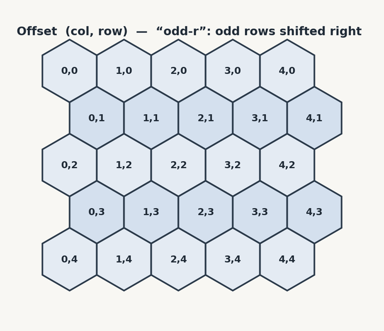
Offset coordinates are great for one thing: dropping a rectangular map straight into a 2D array with no wasted space. They are terrible for everything else. You cannot add two offset coordinates and get a meaningful hexagon, and — as we'll see in §4 — the six neighbor offsets are different on odd and even rows. Any time real math is involved, convert away from offset first.
Cube coordinates — the secret weapon
Here is the idea that makes hexagons easy. Take an ordinary 3D grid of unit cubes, indexed by integers $$$(q, r, s)$$$, and slice it with the diagonal plane $$$q + r + s = 0$$$. The cubes the plane passes through form a perfect hexagonal grid! Each hexagon corresponds to exactly one cube on that plane, and the three coordinate axes of the cube grid become three natural directions on the hex grid.

Why bother carrying three numbers for a 2D grid? Because now hex coordinates behave like ordinary vectors. You can add them, subtract them, scale them by an integer — and every operation automatically lands on another valid hex, as long as you preserve the single constraint $$$q + r + s = 0$$$. All the hard algorithms (distance, rotation, reflection, line drawing) reduce to short, symmetric formulas in cube space. The constraint also guarantees that every hexagon has exactly one canonical coordinate, with no duplicates or gaps.

Axial coordinates — cube without the third wheel
Storing all three cube coordinates is wasteful, because the third is never independent: $$$s = -q - r$$$, always. Axial coordinates simply drop $$$s$$$ and keep $$$(q, r)$$$, recomputing $$$s$$$ in the rare moments an algorithm needs it.

Axial is cube in disguise, so it keeps all the vector goodness — you can add, subtract and scale axial coordinates freely — while using only two integers. This is the system to store hexes in. Think "axial for storage, cube for math," and convert with a one-liner whenever a formula wants $$$s$$$.
Doubled coordinates — the honorable mention
There's a fourth system worth knowing. Doubled coordinates keep (col, row) like offset, but instead of alternating shifts they double one axis' step, enforcing the rule that $$$(col + row)$$$ is even. Unlike offset, doubled coordinates can be added and subtracted safely and have parity-independent neighbors, which makes them a pleasant middle ground for rectangular maps. They're niche in CP, so I'll mention them where relevant but build everything on axial/cube.

Which to use?
Read input in whatever the problem gives you (usually offset). The instant you need to do anything interesting, convert to axial, compute in cube when a formula needs $$$s$$$, and convert back to offset only for output. The conversions are all $$$O(1)$$$ and are the subject of the next section.
3. Conversions between systems
Axial ↔ cube
This pair is trivial and you'll inline it everywhere: to go from axial to cube, recover the missing coordinate; to go back, forget it.
struct Hex  { int q, r; };          // axial
struct Cube { int q, r, s; };       // cube, q+r+s == 0

Cube axial_to_cube(Hex h) { return {h.q, h.r, -h.q - h.r}; }
Hex  cube_to_axial(Cube c) { return {c.q, c.r}; }
Offset ↔ axial
This is the conversion that actually has content, because of the row shift. Each variant (odd-r, even-r, odd-q, even-q) has its own formulas; below is odd-r (pointy, odd rows shoved right), the most common. The r & 1 parity term adds back exactly the half-column that the offset layout shifted away.
Doubled ↔ axial
For completeness, double-width (the pointy-top doubled layout) converts as q = (col - row) / 2, r = row, and back as col = 2q + r, row = r. Double-height swaps the roles.
4. Neighbors and diagonals
The six neighbors
Because axial/cube coordinates are vectors, finding a neighbor is just adding a fixed direction vector — and, crucially, the same six vectors work everywhere on the grid. Going one step in a direction changes one cube coordinate by $$$+1$$$ and another by $$$-1$$$ (so the sum stays $$$0$$$); there are exactly six ways to pick that pair, which is why a hexagon has six neighbors.
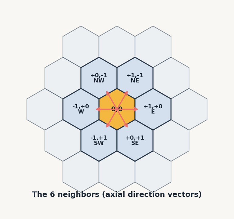
const int DQ[6] = {+1, +1, 0, -1, -1, 0};
const int DR[6] = { 0, -1, -1, 0, +1, +1};
// 0:E  1:NE  2:NW  3:W  4:SW  5:SE   (pointy-top)

Hex neighbor(Hex h, int dir) { return {h.q + DQ[dir], h.r + DR[dir]}; }
Contrast this with offset coordinates, where the six offsets depend on the parity of the row: moving south-east from an even row lands somewhere different (relative to col,row) than from an odd row, so you need two separate lookup tables and a row & 1 branch. That parity headache is the single best reason to never compute on offset coordinates directly.
The six diagonals
Sometimes you want the hexes that touch only at a corner. A diagonal step changes one cube coordinate by $$$\pm 2$$$ and the other two by $$$\mp 1$$$:

const int DIAG_Q[6] = {+2, +1, -1, -2, -1, +1};
const int DIAG_R[6] = {-1, -2, -1, +1, +2, +1};
5. Distances
This is where carrying the third coordinate pays off. Each hexagon maps to a cube in 3D, and two hexagons that are adjacent on the hex grid are distance 2 apart in the cube grid (you change one coordinate by $$$+1$$$ and another by $$$-1$$$, a Manhattan move of 2). So the hex distance is just half the 3D Manhattan distance:
$$$\text{dist}(a,b) = \frac{|a_q-b_q| + |a_r-b_r| + |a_s-b_s|}{2}.$$$
There's an equivalent and often handier form. Because the three differences sum to zero, the largest of them in absolute value always equals the sum of the other two — so the distance is simply the maximum:
$$$\text{dist}(a,b) = \max\big(|a_q-b_q|,\ |a_r-b_r|,\ |a_s-b_s|\big).$$$
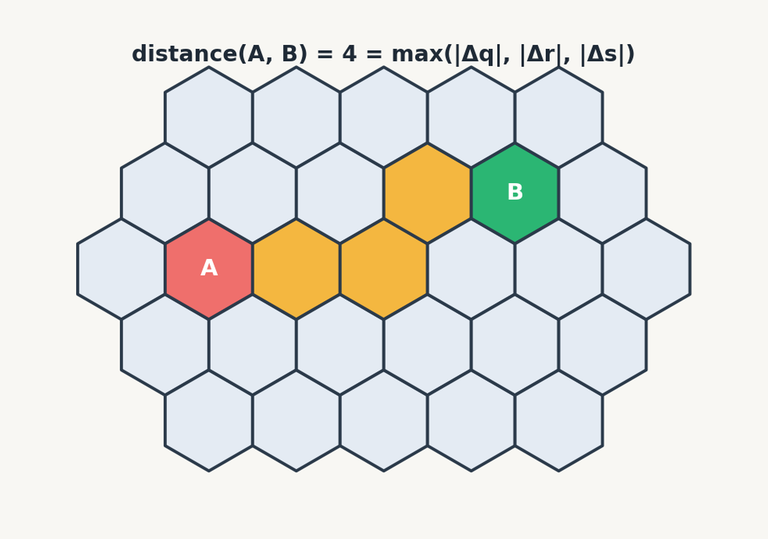
int hex_distance(Hex a, Hex b) {
    int dq = a.q - b.q, dr = a.r - b.r, ds = (-a.q - a.r) - (-b.q - b.r);
    return (abs(dq) + abs(dr) + abs(ds)) / 2;   // == max(|dq|,|dr|,|ds|)
}
You'll see hex distance written a dozen different ways in axial form (the popular "difference of differences" is one of them); every single one is just this cube formula with $$$s$$$ substituted in. If you remember the cube version, you never have to memorize the others.
6. Movement range, intersections, and BFS
All hexes within range N
"Which hexes are at most $$$N$$$ steps away?" Reusing the max-form distance, we need $$$\max(|q|,|r|,|s|)\le N$$$, which means all three of $$$|q|\le N$$$, $$$|r|\le N$$$, $$$|s|\le N$$$ hold simultaneously. Dropping the absolute values gives $$$-N\le q,r,s\le N$$$. The naive triple loop over $$$q,r,s$$$ wastes work because only one $$$s$$$ per $$$(q,r)$$$ satisfies $$$q+r+s=0$$$, so we compute $$$s$$$ directly and let $$$r$$$'s bounds do the clipping:

vector<Hex> hexes_in_range(Hex c, int N) {
    vector<Hex> res;
    for (int dq = -N; dq <= N; dq++)
        for (int dr = max(-N, -dq - N); dr <= min(N, -dq + N); dr++)
            res.push_back({c.q + dq, c.r + dr});
    return res;
}
The number of hexes within range $$$N$$$ is $$$1 + 3N(N+1)$$$ — handy for sizing arrays.
Intersecting two ranges
Each range is the set of hexes satisfying six inequalities of the form $$$q_{\min}\le q\le q_{\max}$$$ (and likewise for $$$r,s$$$). To intersect two hexagonal regions, intersect the intervals coordinate by coordinate — replace each lower bound by the max of the two and each upper bound by the min — then run the same double loop using the tightened bounds. Geometrically you're intersecting two cubes in 3D and projecting the result back onto the plane.
Range with obstacles → BFS
If walls block movement, the clean formula no longer applies and you fall back to a breadth-first search. The good news: BFS on a hex grid is identical to BFS on a square grid — only the neighbor function changes. Expand outward level by level, skipping blocked or already-visited hexes.
7. Line drawing
To list the hexes a straight segment from $$$A$$$ to $$$B$$$ passes through, sample the segment at $$$N+1$$$ evenly spaced points (where $$$N$$$ is the hex distance), then snap each floating-point sample to the nearest hex. The snapping step is cube rounding (§13). This is the hex analogue of the DDA line algorithm.

8. Rotation
Rotating a hex vector (the difference between two hexes) by a multiple of $$$60^\circ $$$ needs no trigonometry at all — it's a signed shuffle of the cube coordinates. A $$$60^\circ $$$ clockwise turn sends $$$(q, r, s)\to(-r, -s, -q)$$$, and counter-clockwise sends $$$(q, r, s)\to(-s, -q, -r)$$$. Apply it $$$k$$$ times for $$$60k$$$ degrees; after six applications you're back where you started.

To rotate a hex around an arbitrary center rather than the origin, do the usual trick: subtract the center, rotate the resulting vector, then add the center back.
9. Reflection
Reflecting a hex across one of the three axes is even simpler: keep the coordinate of the axis you're mirroring over, and swap the other two. Across the $$$q$$$-axis that's $$$(q, r, s)\to(q, s, r)$$$; across $$$r$$$, $$$(q, r, s)\to(s, r, q)$$$; across $$$s$$$, $$$(q, r, s)\to(r, q, s)$$$.

To mirror across a line that doesn't pass through the origin, subtract a reference point on that line, reflect, and add it back — the same shift-and-restore pattern as rotation.
10. Rings and spirals
A single ring
The ring of radius $$$k$$$ is every hex at distance exactly $$$k$$$ from the center. To enumerate it, step $$$k$$$ hexes out to one corner of the ring, then walk along the six edges, taking $$$k$$$ steps on each. After $$$6k$$$ steps you've traced the whole ring and returned to the start.

vector<Hex> hex_ring(Hex center, int k) {
    if (k == 0) return {center};
    vector<Hex> res;
    Hex h = {center.q + DQ[4] * k, center.r + DR[4] * k}; // walk to a corner
    for (int i = 0; i < 6; i++)
        for (int j = 0; j < k; j++) { res.push_back(h); h = neighbor(h, i); }
    return res;
}
(Starting from direction 4 is just a convention that makes the six edges come out in order; pick whatever corner suits your direction numbering.)
Spiraling inward to outward
Concatenate the rings $$$0, 1, 2, \dots, K$$$ and you get a spiral that visits every hex of the big radius-$$$K$$$ hexagon in increasing order of distance — a tidy way to enumerate an area or to assign each hex a single "spiral index."

vector<Hex> hex_spiral(Hex center, int K) {
    vector<Hex> res = {center};
    for (int k = 1; k <= K; k++) {
        vector<Hex> ring = hex_ring(center, k);
        res.insert(res.end(), ring.begin(), ring.end());
    }
    return res;
}
Because ring $$$k$$$ has $$$6k$$$ hexes, the spiral confirms the area formula from §6: $$$1 + 6(1 + 2 + \dots + K) = 1 + 3K(K+1)$$$.
11. Field of view
"What can I see from here, given walls?" The simplest method that actually works: draw a line (§7) from your hex to every hex in range, and call a target visible if its line reaches it without first crossing a wall. It's $$$O(\text{area}\times\text{radius})$$$, which is plenty fast for contest-sized maps and almost impossible to get wrong.

Be aware that "visible" is genuinely ambiguous on grids — center-to-center, any-part-to-any-part, and so on all give slightly different answers, and the simple algorithm occasionally produces a result that looks a little odd near wall corners. Start simple; only reach for a fancier algorithm if a problem's definition forces you to.
12. Hex → pixel and pixel → hex
Hex → pixel
Placing hexes on screen (or recovering real coordinates) comes straight from the spacing in §1. In axial coordinates the position is a linear combination of two basis vectors, one per axis. For pointy-top:
$$$x = \text{size}\cdot\Big(\sqrt{3}\,q + \frac{\sqrt{3}}{2}\,r\Big), \qquad y = \text{size}\cdot\frac{3}{2}\,r.$$$

const double SQ3 = 1.7320508075688772;

pair<double,double> hex_to_pixel(Hex h, double size) {
    double x = size * (SQ3 * h.q + SQ3 / 2.0 * h.r);
    double y = size * (1.5 * h.r);
    return {x, y};
}
If your grid isn't centered at the origin, add an origin offset at the very end; if your hexes aren't square-ish pixels, scale $$$x$$$ and $$$y$$$ independently. Both are easy because the conversion is just a matrix multiply.
Pixel → hex
Going backward — turning a mouse click or a real coordinate into a hex — means inverting that linear map to get a fractional axial coordinate, then rounding it to the nearest real hex. Inverting the matrix gives:
Hex pixel_to_hex(double x, double y, double size) {
    double q = (SQ3 / 3.0 * x - 1.0 / 3.0 * y) / size;
    double r = (2.0 / 3.0 * y) / size;
    Cube c = cube_round(q, r, -q - r);
    return cube_to_axial(c);
}
The rounding step is shared with line drawing and is important enough to get its own section.
13. Rounding a fractional hex
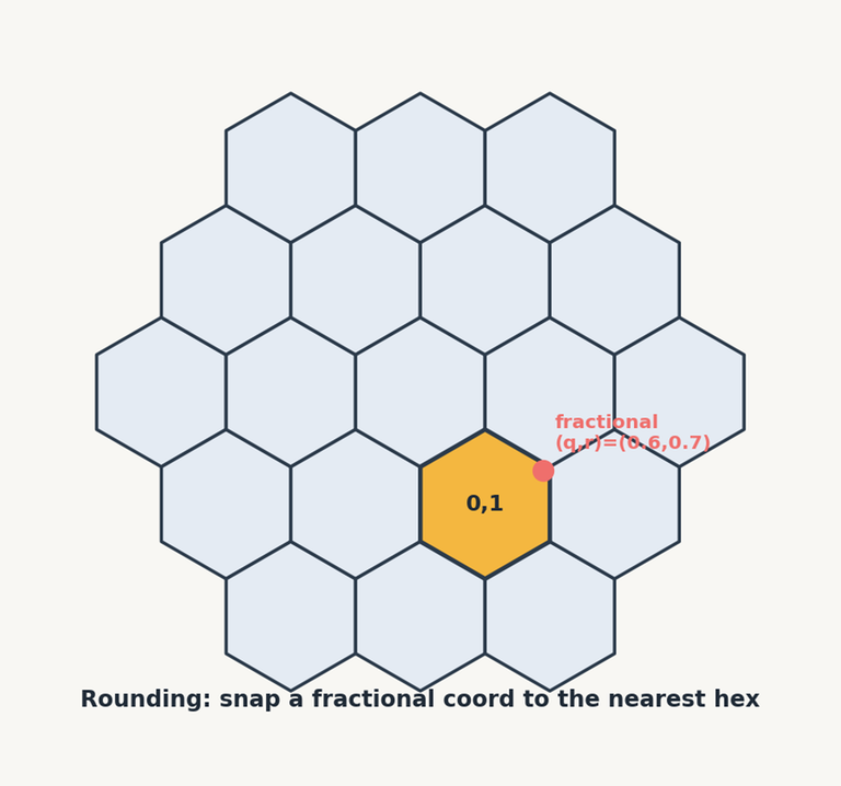
Both line drawing and pixel→hex hand you a floating-point cube coordinate that needs to become an integer hex. Rounding each of $$$q, r, s$$$ to the nearest integer almost works, but the three rounded values might no longer sum to zero. The fix: round all three, then find which one drifted the most from its original value and recompute that one from the other two, restoring $$$q+r+s=0$$$. Resetting the largest-error coordinate guarantees you land in the correct hex.
Cube cube_round(double q, double r, double s) {
    long long rq = llround(q), rr = llround(r), rs = llround(s);
    double dq = fabs(rq - q), dr = fabs(rr - r), ds = fabs(rs - s);
    if (dq > dr && dq > ds) rq = -rr - rs;
    else if (dr > ds)       rr = -rq - rs;
    else                    rs = -rq - rr;
    return {(int)rq, (int)rr, (int)rs};
}
14. Storing a hex map
People worry that axial coordinates "waste" array space, and for a rectangular map they have a point — a naive array[r][q] leaves triangular gaps. Three strategies cover essentially everything.
The first is a plain 2D array with a sentinel in the unused cells; the wasted space is at most a factor of two for common shapes, which is usually not worth optimizing away. The second is a hash map keyed by (q, r), which supports arbitrarily shaped maps — including ones with holes — and is what I reach for most often in contests. The third is to slide each row left and shrink it to its true length so the storage is dense; for a rectangular pointy-top map this means storing hex (q, r) at array[r][q + floor(r/2)], which is exactly the odd-r offset layout.
The practical advice: store coordinates as axial, and hide the storage behind a small getter/setter so the rest of your solution never thinks about it. For a hash key, q * BIG + r with a large constant (or a pair<int,int>) works fine.
15. Wraparound maps
Some problems want the map to wrap, so leaving one edge re-enters from the opposite side. For a hexagon-shaped map of radius $$$N$$$ there are six "mirror" centers arranged around the real one; whenever a computed hex falls off the map, subtract the nearest mirror center to bring it back into the main region. The mirror centers are $$$(2N+1,\,-N,\,-N-1)$$$ in cube coordinates together with its six rotations. The simplest implementation precomputes, for every just-off-the-map hex, its on-map equivalent in a lookup table, and replaces any out-of-range hex via that table.
16. Pathfinding
There is genuinely nothing hex-specific here. A*, Dijkstra and BFS run on hex grids exactly as on square grids; only two pieces plug in differently. The neighbor function is the one from §4 (filter out impassable hexes), and the A* heuristic is the hex distance from §5, scaled to your per-step movement cost — if each hex costs 5 to enter, multiply the distance by 5. Everything else (the priority queue, the came-from map, the path reconstruction) is identical to your square-grid code.
17. A reusable C++ template
Drop this in and you have neighbors, distance, range, lines, rings, rotation and rounding ready for a contest.
To hash hexes in a set/map, key on q * BIG + r or a pair<int,int>.


