Hello Codeforces!

A few months ago, I wrote a blog post about Random heavy light decomposition. Today, I want to discuss a powerful extension of this idea.

How do you usually solve problems where a tree grows online? That is, you process queries that attach a new vertex to the tree, while simultaneously answering queries on paths (e.g., finding the minimum on a path).

Let's try to solve this using Heavy-Light Decomposition (HLD).

The Flaw of Naive HLD

At first glance, one might try a naive approach: when a new vertex is added, simply extend the existing HLD path into it. However, this creates a major vulnerability.

Consider the following case:

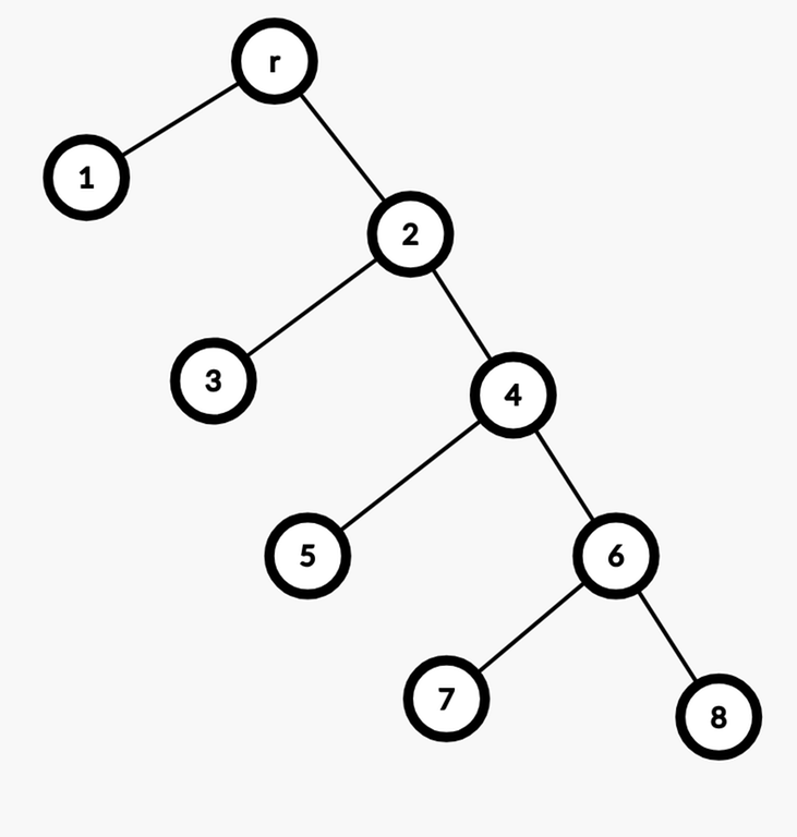
Imagine we repeatedly attach new vertices to form a long path. We extend the HLD path into each of them. But then, we attach a new vertex directly to the root, and subsequently attach all future vertices into its subtree The heavy path we initially built is now useless, and for our new branches, we end up with $$$O(N)$$$ light edges instead of the guaranteed $$$O(\log N)$$$.

One way to fight this is to use query square root decomposition: we can completely rebuild the HLD every $$$\sqrt{Q}$$$ queries. However, this adds an extra $$$O(\sqrt{Q})$$$ factor to our complexity, which is quite unpleasant.

Moreover, intuitively, rebuild entire HLD seems like doing a lot of useless work: most paths aren't touched at all, and those that are touched usually only need updates on a short suffix. We want to rebuild the HLD incrementally, piece by piece, only when absolutely necessary.

An excellent way to achieve this is Randomized HLD.

The Elegance of rnd HLD

Let's assign each vertex a random priority $$$y_v$$$ (e.g., a random integer chosen from $$$[0, 10^9]$$$).

Let $$$smin_v$$$ be the minimum priority $$$y_u$$$ for all $$$u$$$ in the subtree of $$$v$$$, strictly excluding $$$v$$$ itself. We then direct the heavy edge from $$$v$$$ to the child $$$c$$$ whose subtree contains the vertex with priority $$$smin_v$$$.

Proof 1: Expected number of light edges is $$$O(\log N)$$$

Why does this work? Notice that the minimum of $$$S$$$ independent uniform random variables is equally likely to be any of them. Thus, the probability that the minimum priority in $$$v$$$'s subtree falls into the subtree of a specific child $$$u$$$ is exactly $$$\frac{sz_u}{sz_v - 1}$$$.

This means the probability of edge $$$(v, u)$$$ being heavy is exactly proportional to the subtree size! This perfectly reduces to the mathematical proof from my previous blog post:

Thus, the expected number of light edges on any path to the root remains bounded by $$$O(\log N)$$$.

Handling Online Tree Growth

Now, how do we implement the operation of attaching a new vertex new to a parent p?

We simply go up the parent pointers starting from p, as long as $$$smin_{ancestor} \gt y_{new}$$$. Let $$$u$$$ be the highest ancestor we reach where this condition holds. This means $$$y[new]$$$ is now the absolute minimum priority in the subtree of $$$u$$$. We completely rebuild the HLD for the entire subtree of $$$u$$$. For the path that previously went into $$$u$$$, we just update its suffix.

Is this fast enough? Absolutely.

Proof 2: The expected size of the rebuilt subtree is $$$O(\log N)$$$

Let the ancestors of new be $$$p_1, p_2, \dots, p_D$$$ (going up to the root), and let $$$W_k$$$ be the size of $$$p_k$$$'s subtree after adding the new vertex (so $$$W_1 \lt W_2 \lt \dots \lt W_D$$$).

We rebuild the subtree of $$$p_k$$$ if and only if $$$y[new]$$$ is the absolute minimum in the subtree of $$$p_k$$$, but not in the subtree of $$$p_{k+1}$$$. Since $$$y[new]$$$ is a random priority among $$$W_k$$$ vertices, the probability that it is the minimum is $$$\frac{1}{W_k}$$$.

The probability that we rebuild exactly the subtree of $$$p_k$$$ is:

The expected size $$$E$$$ of the rebuilt subtree is the sum of sizes multiplied by their probabilities:

Using the integral bounding technique ($$$\int \frac{1}{x} dx = \ln x$$$):

Therefore, the expected size of the completely rebuilt subtree is bounded by $$$\ln(N) + 1$$$!

Solving the Problem

Let's apply this to a specific task. I started talking about this technique while solving this problem.

Initially, there is a root $$$r$$$ with value $$$a_r$$$. We need to process 3 types of queries online:

1. hang p a_new — attach a new vertex to $$$p$$$ with value $$$a_{new}$$$

2. set v a_new — update $$$a_v := a_{new}$$$

3. get u v x — find the minimum $$$a_s \ge x$$$ where $$$s$$$ lies on the simple path between $$$u$$$ and $$$v$$$

We can solve this using our rnd HLD. To answer the get queries, we need a data structure on each heavy path. We will maintain a Segment Tree where each node contains a std::multiset (a Dynamic Merge Sort Tree).

Let's calculate the expected time complexity for each operation:

• set v a_new: The vertex $$$v$$$ belongs to exactly one heavy path. A point update in a Segment Tree of multisets requires updating $$$O(\log N)$$$ nodes. In each node, we erase the old value and insert the new one in $$$O(\log N)$$$ time. Time: $$$O(\log^2 N)$$$ expected.

• get u v x: Thanks to rnd HLD, the path is split into $$$O(\log N)$$$ expected heavy path segments. On each segment, we query the Segment Tree, covering $$$O(\log N)$$$ nodes. Inside each of these nodes, we find the answer via multiset::lower_bound in $$$O(\log N)$$$. Time: $$$O(\log^3 N)$$$ expected.

• hang p a_new: We just proved the expected size of the rebuilt subtree is $$$W \le \ln(N) + 1$$$. Rebuilding the HLD structure takes $$$O(W)$$$. Rebuilding the Segment Tree of multisets for paths of total length $$$W$$$ takes $$$O(W \log W)$$$ (if we build it bottom-up). The expected rebuild time is $$$ \sum P_k \cdot O(W_k \log W_k) \le O(\log N) \sum P_k W_k = O(\log N) \cdot O(\log N) $$$ Time: $$$O(\log^2 N)$$$ expected.

Compared to standard query square root decomposition which would work in $$$O(N \sqrt{Q} \log N + Q log ^ 3 N)$$$, our rnd HLD achieves a clean $$$O(Q \log^3 N)$$$ overall with excellent constant factors and avoids any blocking logic!

Thus, rnd HLD is indeed a very useful technique for dynamic tree problems.

Thank you for reading the post!