Hi there!

Some long time ago, I and SashaT9 thought of an idea to create a collection of little tricks useful in competitive programming. We believe that such a website can both boost beginners, and be useful for experts as a reference website containing many example problems, which can be used, for example, to recall something, or, say, make an educational contest.

It worth to say that there are already a bunch of blogs here with the same purpose. Our main feature is that we provide not just a list of tricks with their brief descriptions, but a detailed pages for each of them.

This project was inspired by tricki (currently dead) project. I already posted a test blog in order to demonstrate this format here.

We run a website based upon mkdocs (similar to cp-algorithms):

https://cp-tricki.github.io/

Now we wrote five more or less simple (but unfortunately unpolished) pages:

1. Counting labeled trees
2. One can process bits independently when relevant
3. Permutations can be represented as graphs
4. Translate DP to the matrix form
5. How to come up with a comparator?
6. (02.10.23) One can use determinants to count lattice paths
7. (02.10.23) Small number of groups can be processed straightforwardly
8. (03.10.23) Use diagonals as parameters in grid DP problems
9. (03.10.23) How to use ternary search
10. (03.10.23) Lagrange multipliers can simplify tricky optimisation problems

This is an open project, so we encourage everybody to write their expositions and make add them to the github repository.

Miaow! Miaow! =^◡^=

This is a cp-tricki article, inspired by the dead project tricki. The idea of the project is to publish short blogs elaborating on ideas that are too small or simple for a comprehensive tutorial, but still useful for many people.

We do not claim any authorship of these tricks, taking our primary purpose to popularise them, so we hope that somebody will find these ideas fruitful.

Acknowledgements.

We start from a simple trick, which was exposed by Sergei Kopeliovich at Winter Programming School in Kharkiv in 2013.

Short description.

If it seems that a problem can be solved by an algorithm of the form: "arrange the objects in a suitable way and then work greedily", there is a general strategy to devise a comparator for this sort.

Prerequisites.

No specific knowledge is required, though familiarity with greedy algorithms would be useful.

General description

The auxiliary problem: find an order that optimises a construction (that is the essential part of the considered problem) if it is known that such an order exists.

We first consider a simplified problem, when only two objects exist, say $$$A$$$ and $$$B$$$. Then our comparator should determine which order is better: $$$AB$$$ or $$$BA$$$. To do so, we can normally introduce a penalty (or a cost) function $$$f(A,B)$$$ denoting the amount of penalty (or cost) we have if one takes object $$$A$$$ first and object $$$B$$$ second. Then our comparator chooses that order in which the penalty is minimal (or cost is maximal). If this comparator (relation) $$$A\prec B$$$ (which is $$$A\prec B \iff penalty(A,B)<penalty(B,A)$$$ or $$$cost(A,B)>cost(B,A)$$$) is transitive (i.e. if $$$A\prec B$$$ and $$$B\prec C$$$ then $$$A\prec C$$$) then after sorting all the objects with respect to it we shall obtain the optimal order.

The main problem: find a maximal-size subset that optimises a construction. (The difference from idea 1 is that we are not forced to take all elements.)

To do so, we use the comparator from the auxiliary problem, and take objects greedily one by one. At each step, we make a choice:

1. Put this object into the answer set,

2. Replace an instance in the answer set with this object.

More generally one can write here a knapsack-like dp (if we have a subset we know the order by the auxiliary problem).

Example 1.

Given $$$n$$$ boxes, each of which has its weight $$$m_i$$$ and the weight it can carry on the top $$$a_i$$$, determine the size of the largest tower one can build.

Example 2 (this CSES problem).

Given $$$n$$$ people and their programmer skill ($$$skill_1$$$) and artistic skill ($$$skill_2$$$). We need to take exactly $$$a$$$ programmers and $$$b$$$ artists. Maximise total skill.

Online Judges

1. https://www.eolymp.com/en/problems/4701 (problem from Example 1, only Russian statement available)
2. https://www.eolymp.com/en/problems/9640
3. https://www.eolymp.com/en/problems/1591
4. https://www.eolymp.com/en/problems/2219
5. https://www.eolymp.com/en/problems/4699 (only Russian statement available)
6. https://codeforces.me/gym/104397/problem/A

Hello, Codeforces!

1. Recently, adamant published an excellent blog Stirling numbers with fixed n and k. There he described an approach to them via generating functions.

In this (messy) blog, I want to share one useful technique on the example of Stirling numbers of the first kind.

2. We start with the definition of the Stirling transformation of a sequence $$$(x_n)$$$ is the following mapping

where $$$s(n,k)$$$ is a first-kind Stirling number. Here we have a place of flexibility for our technique: we can choose any other function $$$f(n,k)$$$ instead of Stirling numbers, though it only sometimes turns out to be useful.

3. The essence of this method is to find the transition formulae between Stirling transformations of a sequence $$$(x_n)$$$ and the sequence of its finite differences (one can think of it as a discrete analogue of derivative) $$$(y_n)$$$ defined by

The acquaintance with finite differences is highly recommended for the readers of this blog.

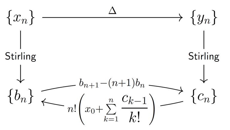
Theorem 1 (Transition formulae). In fact, the following transition formulae hold:

Step 1. How to work with finite differences?

Theorem 2 (solving first-order linear difference equation). Let $$$(y_k)$$$ be a recurrence relation that satisfies

where $$$(p_k), (q_k)$$$ are given sequences and there is no $$$i$$$ such that $$$p_i=0$$$, then the solution to this equation is given by

Step 2. Proof of the Theorem 1.

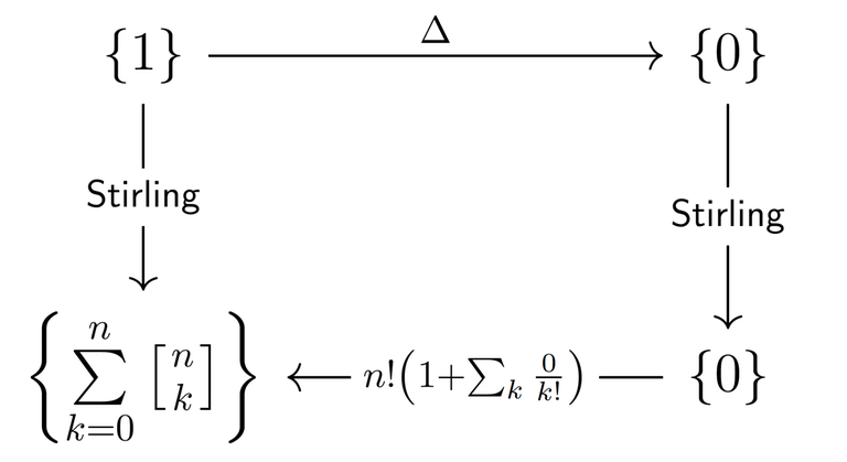
4. Using these transition formulae we can derive countless identities with Stirling numbers of the first kind (as well as identities involving binomial coefficients and other interesting combinatorial functions, as pointed out in 2). For example, taking $$$x_n = 1$$$, we obtain the following nice identity

visualised by the diagram

5. A nontrivial and interesting example. We exploit the combinatorial nature of $$$s(n,k)$$$ to write down the average number of cycles in a random permutation.

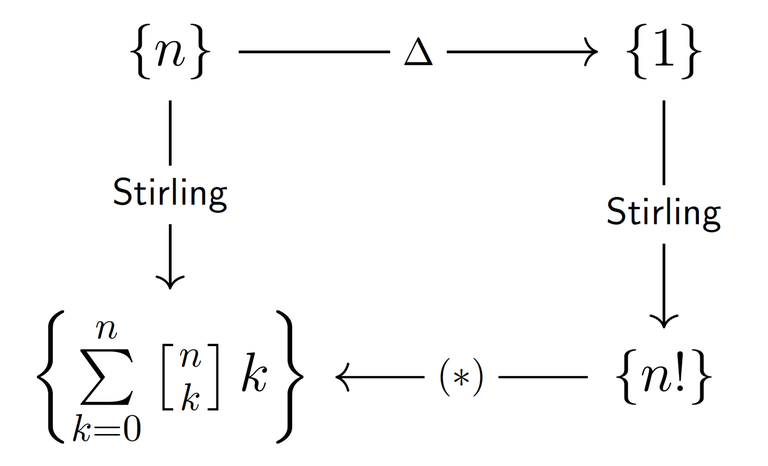
We can easily find the sum in the numerator by applying theorem 1 to the sequence $$$x_n = n$$$.

where $$$H_n = 1 + 1/2 + \dots + 1/n$$$ is $$$n$$$-th Harmonic number. Hence $$$\mathbf{E}[cycles]=H_n=O(\log n)$$$, a very nice result!

6. We generalise 5 and 6 by consider the sequence $$$x_n = n^k$$$ for a fixed $$$k$$$. From adamant's blog (highly connected with this section), we know that first-kind Stirling numbers behave much better with falling factorials. So, in order to find a good formula for the Stirling transformation of $$$n^k$$$, we first find it for $$$(n)_k$$$ and then apply

and derive the desired formula.

The details are left for the reader, here is the outline.

Step 1. Prove the identity $$$\sum_{j=0}^{N} s(j,k)/j! = 1/N! s(N+1,k+1)$$$ by double induction and Pascal-like identity (lemma 1).

Step 2. Apply Theorem 1 to $$$x_n=(n)_k$$$ (fix $$$k$$$) and using 1 prove that

Step 3. Finally, prove that

The last formula is obviously practical.

7 (Bonus).

Theorem 3 (transition between two kinds of Stirling numbers). Let $$$(a_n)$$$ be a sequence and

be is second-kind Stirling transform. Then

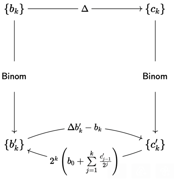
8 (Remark). I mentioned twice that this method can be generalised. For example, for the binomial transformation

the main theorem will be the following

Using a similar strategy as in 6, we can prove that

In August 2022, I had a talk concerning lattice paths at a summer programming school in Khust, Ukraine. After, I realised that some aspects of my talk aren't well-known in the CP community and, in this blogpost, I'd like to very briefly and untidily (so feel free to ask for additional explanations by comments) share the main points of that talk.

I hope that ideas presented in the blog will help you sometime.

1. Lattice paths

1.1. Walks without restrictions.

1.1.1. We start from a rudimentary example. Consider a $$$N\times M$$$ grid and a robot (or a chip, or a ship, or anything else you wish) at $$$(0,0)$$$ (not a cell, an intersection point) which can move in the east unit direction and in the north unit direction. A route that the robot is able to make is said to be northeastern. How many northeastern paths are there? In fact, We can bijectively code any path with a corresponding string of the form $$$\uparrow\rightarrow\rightarrow\rightarrow\uparrow\rightarrow\dots$$$ of length $$$N+M$$$. There are $$$N$$$ places to put $$$\rightarrow$$$ hence there are $$$\binom{N+M}{N}$$$ such paths.

1.1.2. One can easily generalise this formula to a $$$d$$$-dimensional case. Indeed, consider a $$$d$$$-dimensional box (grid) $$$[N_1]\times [N_2]\times \dots\times [N_d]$$$ (where $$$[M] = {1,\dots,M}$$$). Then, the robot can make steps which are from the orthonormal basis i. e. $$$\mathbf{e}_1=(1,0,\dots,0)$$$, $$$\mathbf{e}_2=(0,1,\dots,0)$$$, $$$\dots$$$, $$$\mathbf{e}_d = (0,0,\dots,1)$$$. Then, the string consists of the numbers between $$$1$$$ and $$$d$$$ which represent the steps of the robot. We have $$$N_1+\dots+N_d$$$ steps in total: $$$N_1$$$ steps correspond to $$$\mathbf{e}_1$$$, $$$N_2$$$ steps correspond to $$$\mathbf{e}_2$$$, etc. There are $$$N_1+N_2+\dots+N_d$$$ "free" seats for the steps of the first kind, $$$N_2+\dots+N_d$$$ `free' seats for the steps of the second kind and etc. Hence, there are

paths. One may do some algebra and obtain a splendid formula which, in fact, is a multinomial coefficient that appears in a generalisation of the binomial theorem

1.1.2*. It is worth saying several words about a geometric interpretation of the multinomial theorem. For the sake of exposition, the only case we explain is $$$d=2$$$, just because we can simply draw and imagine it. Consider an infinite grid with origin $$$(0,0)$$$ and with blue horizontal and red vertical lines. Let the cost of the blue unit segment be $$$a$$$ and the cost of the red unit segment be $$$b$$$ (as monomials, not numbers). The cost of a path is a product of all the unit segments in it. That is the cost of a path which consists of 4 horizontal and 3 vertical unit steps is $$$a^4b^3$$$. So,

The $$$d$$$-dimensional formula is

1.2. Catalan numbers

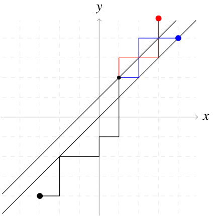
1.2.1 Almost everyone knows about Catalan numbers, yet, as a prelude we demonstrate the first implementation of the reflection method (André reflection method), we shall write a bit about the combinatorial derivation of the closed form. Indeed, the first natural question, after 1.1 is about the number of paths under some restrictions. How many northeastern paths from $$$(a,b)$$$ to $$$(c,d)$$$ which lie under $$$y=x$$$ are there (we additionally assume $$$a\geq b$$$ and $$$c\geq d$$$ to avoid pitfalls).

1.2.2. The first caveat is that it is allowed to touch $$$y=x$$$, which, in fact, is an intersection. Instead, we consider a shifted line $$$y=x+1$$$. Then, any intersection (including touching) with $$$y=x+1$$$ is forbidden and now we can safely touch the line $$$y=x$$$. We also shall count the number of bad paths (which intersects $$$y=x+1$$$) and then we shall just subtract this number from the total one: $$$\binom{c-a+d-b}{c-a}$$$ (according to 1.1).

1.2.3. Consider any bad path from $$$(a,b)$$$ to $$$(c,d)$$$ (such path exists because of $$$a\geq b$$$ and $$$c\geq d$$$) and the first intersection point with $$$y=x+1$$$. Reflect this path with respect to this line and we thus obtain a bad path from $$$(a,b)$$$ to $$$(d-1,c+1)$$$. Moreover, any path from $$$(a,b)$$$ to $$$(d-1,c+1)$$$ definitely intersects $$$y=x+1$$$ and therefore is bad. So, we obtained the bijection between bad paths and all paths between $$$(a,b)$$$ and $$$(d-1,c+1)$$$. There are exactly, again by 1.1, $$$\binom{c-a+d-b}{c-b+1}$$$ such paths.

Therefore, the number of under-$$$y=x$$$ paths is equal to

In particular, when $$$a=b=0$$$ and $$$c=d=N$$$ we obtain

2. The reflection method on graphs

This section will be about Lindstrom-Gessel-Viennot lemma, yet for the sake of exposition, we present a non-weighted version.

2.1.1. Definitions

2.1.1. Let $$$G$$$ be an oriented acyclic graph. Consider two sets of vertices

Note that $$$n$$$ is the same for both sets.

2.1.2. Introduce a path matrix $$$M_G(\mathbf{A},\mathbf{B})$$$ (when one can easily recover $$$G$$$, $$$\textbf{A}$$$ and $$$\mathbf{B}$$$ from the context, we shall abridge the notation and simply write $$$M$$$). Let $$$M_{ij}$$$ be equal to the number of paths from $$$A_i$$$ to $$$B_j$$$. Note that this number is well-defined since $$$G$$$ is acyclic.

2.1.3. A path system $$$\mathbf{P}_\pi (\mathbf{A}, \mathbf{B})$$$ (where $$$\pi$$$ is a permutation of $$${1,\dots,n}$$$) is a set of paths

Note that the existence of multiple paths between two vertices is possible, and consequently, it's not guaranteed that a path system is unique. A path system is said to be disjoint if there is no vertex which belongs to two or more paths.

2.2. Unweighted LGV-lemma

2.2.1. We are ready to state the unweighted LGV-lemma.

Lemma. For any acyclic oriented graph $$$G$$$ and two sets (of the same size) $$$\mathbf{A}, \mathbf{B}$$$ of its vertices it holds that

2.2.2. We write the definition of determinant.

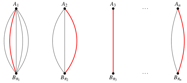
Recall that $$$M_{1\pi_1}$$$ is the number of paths from $$$A_1$$$ to $$$B_{\pi_1}$$$, ..., $$$M_{n\pi_n}$$$ is the number of paths from $$$A_n$$$ to $$$B_{\pi_n}$$$. Their product $$$M_{1\pi_1} M_{2\pi_2} \dots M_{n\pi_n}$$$ is the total number of paths systems with the fixed permutation $$$\pi$$$. See the picture below.

Therefore, we obtain the following formula

2.2.3. In 2.2.2 we proved that sum of signs over all path systems is equal to the determinant. So, the rest is to prove

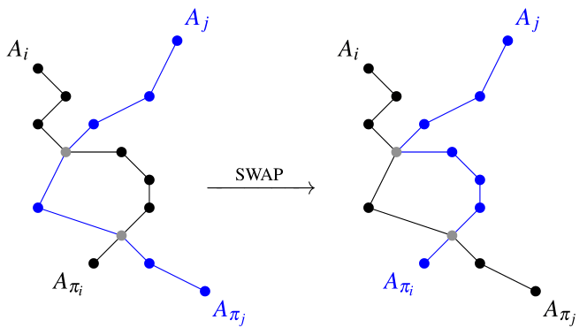
2.2.4. Let $$$\mathbf{P}_\pi$$$ be an intersecting path system. Consider the smallest `bad' $$$i$$$ such that $$$A_i \to B_{\pi_i}$$$ shares some vertex. Let $$$X$$$ be the first such vertex and $$$j$$$ be the smallest $$$j>i$$$ such that path $$$A_j \to B_{\pi_j}$$$ contains $$$X$$$. We construct a new path system by swapping:

And the picture:

2.2.5. The rest is the analysis of this highly elegant construction. However, we prefer to incautiously say that it's an involution and hence a bijection on the set of intersecting path systems, yet one may check it explicitly and carefully. Moreover, SWAP makes a transposition and hence changes the parity of the permutation $$$\pi$$$. So,

And hence the claim asked in 2.2.3 holds. Congratulations, your repertoire was enhanced with LGV-lemma!

3. Applications

3.1. The very first application

The graph, in this section, is just a large portion of the northeastern infinite grid graph.

3.1.1. Let $$$a_1<\dots<a_N$$$ and $$$b_1<\dots<b_N$$$ be sequences of nonnegative integers. Then the number of paths systems from $$$\mathbf{A} = {(0,a_i)}$$$ to $$$\mathbf{B} = {(K,b_i)}$$$ (where $$$K$$$ is some fixed number) can be computed as determinant

Indeed, since $$$a_1<\dots<a_N$$$ and $$$b_1<\dots<b_N$$$ the only one disjoint paths system is identity system: $$$A_i \to B_i$$$ for all possible $$$i$$$. The rest is the application of LGV-lemma. An example problem: 348D - Turtles.

3.1.2. Another variation of the first example is the following: how many paths $$$(0,0)$$$ to $$$(N,M)$$$ are there if it's forbidden to touch any of given $$$K$$$ points, say $$$(x_1,y_1)$$$, ..., $$$(x_K, y_K)$$$?

Introduce two sets $$$\mathbf{A} = ((0,0); (x_1,y_1); \dots; (x_K,y_K))$$$ and $$$\mathbf{B} = ((N,M); (x_1,y_1); \dots; (x_K,y_K))$$$. It's easy to realise that any disjoint paths system is identity one. Since it's disjoint we can intersect (and particularly even touch) paths $$$(x_i,y_i)\to (x_i,y_i)$$$, which, in fact, are our forbidden points. So, the answer to the problem is $$$\det M(\mathbf{A},\mathbf{B})$$$.

3.2. Plane partitions

3.2.1. How many plane partitions in a box $$$a\times b\times c$$$ are there?

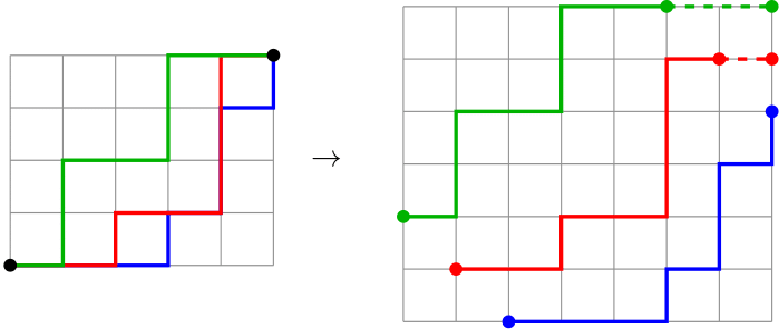
3.2.2. Recall, that plane partition is just a chain of included Young diagrams. Yet, a Young diagram is just a lattice path. So, a plane partition is just a collection of `almost disjoint paths. We shift these paths in order to obtain a disjoint paths system.

So,

The rest is the algebra:

Use Pochhammer symbols:

This one is, in fact, Vandermonde determinant, which can be evaluated explicitly:

We can continue

Return back,

So, the final $$$O(a+b+c)$$$ formula is

3.3. Miscellaneous

This `reflection method' can be used to prove hook-length formula.

You can also can enjoy with one more problem from AtCoder.