Hello Codeforces!

Pascal's Triangle is one of the first concepts we encounter in combinatorics. On the surface, it looks trivial, just a simple addition grid. However, in competitive programming, problem setters love to twist its properties, sum its elements along weird paths, or throw massive constraints at you that break standard algorithms.

Whether you are a beginner looking to understand the fundamentals or a Div. 1 veteran preparing for extreme variations involving composite moduli, this blog is your one-stop reference.

1. Foundations & Intuition

Pascal's Triangle is a geometric representation of binomial coefficients. The value at the $$$n$$$-th row and $$$k$$$-th column (0-indexed) corresponds exactly to $$$\binom{n}{k}$$$ (or $$$nCr$$$), representing the number of ways to choose $$$k$$$ elements from a set of size $$$n$$$.

The entire triangle is built upon a single, intuitive recurrence relation:

       

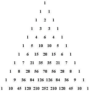
Basic $$$O(N^2)$$$ Matrix Implementation

When $$$N \le 2000$$$, we can precompute the matrix. This is incredibly robust because it handles any modulus (prime or composite) without needing modular inverses, preventing division-by-zero errors.

const int MAXN = 2000;
const int MOD = 1e9 + 7;
int C[MAXN + 1][MAXN + 1];

void precompute_pascal() {
    for (int i = 0; i <= MAXN; i++) {
        C[i][0] = 1;
        for (int j = 1; j <= i; j++) {
            C[i][j] = (C[i - 1][j - 1] + C[i - 1][j]) % MOD;
        }
    }
}

2. Powerful Identities (The $$$O(1)$$$ Optimization Hacks)

If your solution requires looping over combinations, you can almost always use a property of Pascal's Triangle to reduce that loop to an $$$O(1)$$$ calculation.

A. Row Sums (Total Subsets)

The sum of all elements in the $$$n$$$-th row is always $$$2^n$$$:

B. The Hockey Stick Identity

If you sum elements along a diagonal starting from the boundary 1, the total equals the element directly below and turned inward.

CP Application: Essential for optimizing DP state transitions where you are required to sum a prefix of combinations.

C. Symmetry

Choosing $$$k$$$ items to keep is identical to choosing $$$n-k$$$ items to reject:

3. Scaling Up: Advanced Constraints & Prime Moduli

When $$$N$$$ and $$$K$$$ grow up to $$$10^6$$$ or $$$10^{18}$$$, the $$$O(N^2)$$$ grid fails due to both Time Limit Exceeded (TLE) and Memory Limit Exceeded (MLE).

Variation 1: $$$N, K \le 10^6$$$, Modulo is a Large Prime ($$$M = 10^9+7$$$)

Instead of the grid, we use the factorial definition: $$$\binom{n}{k} = \frac{n!}{k!(n-k)!}$$$. We precompute factorials and their modular inverses using Fermat's Little Theorem ($$$A^{-1} \equiv A^{M-2} \pmod M$$$) in $$$O(N)$$$ time, allowing $$$O(1)$$$ queries.

long long fact[MAXN + 1], invFact[MAXN + 1];

long long power(long long base, long long exp) {
    long long res = 1;
    base %= MOD;
    while (exp > 0) {
        if (exp % 2 == 1) res = (res * base) % MOD;
        base = (base * base) % MOD;
        exp /= 2;
    }
    return res;
}

void precompute_factorials() {
    fact[0] = 1;
    invFact[0] = 1;
    for (int i = 1; i <= MAXN; i++) fact[i] = (fact[i - 1] * i) % MOD;
    invFact[MAXN] = power(fact[MAXN], MOD - 2);
    for (int i = MAXN - 1; i >= 1; i--) invFact[i] = (invFact[i + 1] * (i + 1)) % MOD;
}

long long nCr(int n, int k) {
    if (k < 0 || k > n) return 0;
    return fact[n] * invFact[k] % MOD * invFact[n - k] % MOD;
}

Variation 2: Massive $$$N \le 10^{18}$$$, Modulo is a Small Prime ($$$P \le 10^5$$$)

When $$$N$$$ is massive, you cannot precompute factorials up to $$$N$$$. Furthermore, since $$$N \ge P$$$, factorials will contain multiples of $$$P$$$, resulting in $$$0$$$ or division-by-zero errors.

Lucas' Theorem saves us here. It states that we can break $$$\binom{n}{k}$$$ down by converting $$$n$$$ and $$$k$$$ into their base-$$$P$$$ representations:

Where $$$n_i$$$ and $$$k_i$$$ are the digits of $$$n$$$ and $$$k$$$ in base $$$P$$$.

long long nCr_lucas(long long n, long long k, int p) {
    if (k == 0) return 1;
    long long ni = n % p;
    long long ki = k % p;
    if (ni < ki) return 0;
    
    // small_nCr uses the standard O(P) factorial array
    return (small_nCr(ni, ki, p) * nCr_lucas(n / p, k / p, p)) % p; 
}

Complexity: $$$O(P)$$$ initialization + $$$O(\log_P N)$$$ per query.

4. The Final Boss: $$$\binom{n}{k} \pmod M$$$ where $$$M$$$ is Composite

What if $$$N, K \le 10^{18}$$$, but $$$M$$$ is not prime (e.g., $$$M = 10^6$$$ or a random composite number)? Fermat’s Little Theorem fails because modular inverses don't exist for numbers that share factors with $$$M$$$. Lucas' Theorem also fails because it strictly requires a prime base.

To solve this, we use a three-step mathematical pipeline: Prime Factorization $$$\rightarrow$$$ Legendre's Formula + Prime Power Solving $$$\rightarrow$$$ Chinese Remainder Theorem (CRT).

Step 1: Factorize $$$M$$$ into Prime Powers

We break $$$M$$$ into its unique prime power components:

We will calculate $$$R_i = \binom{n}{k} \pmod{{p_i}^{e_i}}$$$ separately for each prime power, and then combine them at the end.

Step 2: Computing $$$\binom{n}{k} \pmod{p^e}$$$

To compute $$$\frac{n!}{k!(n-k)!} \pmod{p^e}$$$, we cannot include any multiples of $$$p$$$ in our factorial calculations because they do not have modular inverses.

Instead, we extract the prime $$$p$$$ completely from the factorials. We can rewrite any integer $$$x!$$$ as:

Where $$$v_p(x!)$$$ is the number of times $$$p$$$ divides $$$x!$$$ (calculated in $$$O(\log_p x)$$$ time using Legendre's Formula):

And $$$m_x$$$ is the remaining product of all numbers up to $$$x$$$ with all factors of $$$p$$$ divided out. Since $$$\gcd(m_x, p^e) = 1$$$, $$$m_x$$$ possesses a valid modular inverse!

Thus, we can evaluate the combination cleanly:

Step 3: Combine with the Chinese Remainder Theorem (CRT)

Once we have calculated a system of congruences:

We use the standard Chinese Remainder Theorem to find a unique solution for $$$x$$$ modulo $$$M$$$.

Summary Matrix of Approaches

5. Practice Problems

• CSES Task 1715 — Creating Strings II
• CSES Task 1716 — Distributing Apples
• Codeforces 1850F — We Were Here Together
• Codeforces 1244C — The Football Season

Mastering these transitions will ensure that no matter how a problem setter limits your memory or runtime, you can exploit Pascal's properties to secure an Accepted verdict.

Feel free to drop any questions or link relevant problems in the comments below!

Hello Codeforces!

Combinatorics and counting problems are a staple in competitive programming. Today, I want to discuss a classic yet incredibly powerful concept that frequently appears in $$$O(N)$$$ DP optimizations and math-heavy problems: Derangements.

Whether you are grinding Div. 2 B/C problems or tackling high-level combinatorics on USACO and AtCoder, understanding the intuition behind derangements is a massive advantage. Let's dive in!

1. What is a Derangement?

A derangement is a permutation of the elements of a set such that no element appears in its original position.

If we have an array $$$A = [1, 2, 3, \dots, N]$$$, a derangement is a permutation $$$P$$$ where $$$P[i] \neq i$$$ for all $$$1 \le i \le N$$$.

Classic Examples: * Secret Santa: $$$N$$$ people put their names in a hat and each draws one. A valid state is when nobody draws their own name. * The Hat-Check Problem: $$$N$$$ guests check their hats. The attendant hands them back randomly. What is the probability nobody gets their own hat?

The number of derangements of a set of size $$$N$$$ is denoted as $$$!N$$$ (read as subfactorial $$$N$$$) or $$$D_n$$$.

2. The Core Mathematics & Recurrences

To solve this efficiently, we don't generate permutations. Instead, we rely on recurrence relations.

Recurrence 1: The Intuitive Approach

The most standard recurrence for derangements is:

Proof / Intuition: Imagine $$$N$$$ people. Let person $$$1$$$ take the spot of person $$$i$$$ ($$$2 \le i \le n$$$). There are exactly $$$(n - 1)$$$ choices for $$$i$$$. Now, what does person $$$i$$$ do? 1. Case 1 (They swap): Person $$$i$$$ takes person $$$1$$$'s original spot. The two people have perfectly swapped. The remaining $$$(n - 2)$$$ people must now be deranged among themselves. This gives $$$D_{n-2}$$$ ways. 2. Case 2 (They don't swap): Person $$$i$$$ does not take person $$$1$$$'s spot. This is mathematically identical to saying person $$$i$$$ is forbidden from exactly one specific spot (spot 1), while the other $$$(n-2)$$$ people are forbidden from their own spots. This maps perfectly to a derangement problem of size $$$(n - 1)$$$. This gives $$$D_{n-1}$$$ ways.

Summing these cases and multiplying by the $$$(n - 1)$$$ choices yields our formula!

Recurrence 2: The Linear Step

A tighter recurrence relation exists, which is incredibly useful for space optimization:

The Closed Form (Inclusion-Exclusion)

Using the Principle of Inclusion-Exclusion (PIE), the exact formula is:

(Fun fact: As $$$n \to \infty$$$, the probability of a random permutation being a derangement approaches $$$\frac{1}{e} \approx 36.78\%$$$.)

3. Implementation (C++)

In CP, we usually need to compute $$$D_n \pmod M$$$ (where $$$M = 10^9+7$$$ or $$$998244353$$$).

Approach A: $$$O(N)$$$ Precomputation

Perfect when you need to answer multiple test cases. Space Complexity: $$$O(N)$$$. Time Complexity: $$$O(N)$$$.

#include <iostream>
#include <vector>

using namespace std;

const int MOD = 1e9 + 7;
const int MAXN = 1e6;

vector<long long> D(MAXN + 1);

void precompute() {
    D[0] = 1; // Base case: 1 way to derange 0 elements
    D[1] = 0; // Base case: 0 ways to derange 1 element
    
    for (int i = 2; i <= MAXN; ++i) {
        D[i] = (i - 1) * (D[i - 1] + D[i - 2]) % MOD;
    }
}

void solve() {
    int n;
    cin >> n;
    cout << D[n] << "\n";
}

int main() {
    ios_base::sync_with_stdio(false);
    cin.tie(NULL);
    precompute();
    
    int t;
    cin >> t;
    while (t--) {
        solve();
    }
    return 0;
}

Approach B: $$$O(1)$$$ Space Optimization

If you only need to query $$$D_n$$$ once for a massive $$$N$$$, you can roll the variables just like the Fibonacci sequence. Space Complexity: $$$O(1)$$$.

long long get_derangement(int n) {
    if (n == 0) return 1;
    if (n == 1) return 0;
    
    long long prev2 = 1; // D[0]
    long long prev1 = 0; // D[1]
    long long current = 0;
    
    for (int i = 2; i <= n; ++i) {
        current = (i - 1) * (prev1 + prev2) % MOD;
        prev2 = prev1;
        prev1 = current;
    }
    return current;
}

4. Advanced Variations (For Div 1 / Hard Div 2)

Partial Derangements (Rencontres Numbers): What if a problem asks: "How many permutations exist where exactly $$$K$$$ elements are in their original positions?"

You choose which $$$K$$$ elements stay in place, and then completely derange the remaining $$$N - K$$$ elements:

Massive $$$N$$$ Queries using NTT: If $$$N \ge 10^5$$$ and the modulus allows, you can view the closed-form PIE formula as a convolution of two polynomials: $$$A[i] = \frac{(-1)^i}{i!}$$$ and $$$B[j] = j!$$$. This allows computing the entire array using Number Theoretic Transform (NTT) in $$$O(N \log N)$$$ time, though standard $$$O(N)$$$ is almost always sufficient unless there's a strict time limit on array generation.

5. Practice Problems

• CSES Task 1717 — Christmas Party
• Codeforces 1530D — Secret Santa
• Codeforces 340E — Iahub and Permutations

I hope this guide helps solidify your understanding of derangements! Feel free to ask questions in the comments or point out any other interesting problems that use this concept.

Happy coding!