Блог пользователя PurpleCrayon

Автор PurpleCrayon, 2 года назад, По-английски

hi

Today's post continues my theme of niche but sometimes useful topics in CP. This idea was brought to my attention by magnus.hegdahl, so thanks to him!

General Description

The motivation behind the technique is to solve the following problem: Given a static array $$$a$$$ of $$$n$$$ elements (for convenience, I'll assume $$$n$$$ is a power of $$$2$$$, if not, the array can be padded with null elements), answer $$$q$$$ queries of the form $$$($$$$$$l$$$, $$$r$$$, $$$x$$$$$$)$$$ where you have to print $$$\sum\limits_{k = l}^r a_{k \oplus x}$$$. In particular, a query where $$$x = 0$$$ is just a normal segtree query. If $$$x$$$ is non-zero, the array indices that are being queried are no longer contiguous, making this impossible to solve with a normal segtree. Note: the only requirement is that the "addition" operation is associative (commutativity is not required). The solution provided in this blog solves the problem in $$$\mathcal{O}(n \log{} n + q \log{} n)$$$ with $$$\mathcal{O}(n \log{} n)$$$ memory. The memory can be reduced to $$$\mathcal{O}(n)$$$ if the "addition" operation is commutative.

About the name: I've seen it called XOR segment tree in 2 different places, so I assume that's what people know it as. Let me know if you've seen it being called something else.

For the rest of this tutorial, I will assume that you use a recursive implemenetation of segment trees.

Commutative case

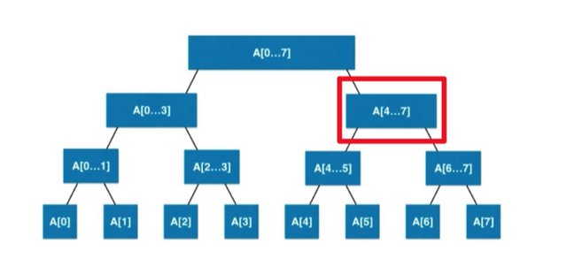
To start off, let's solve the commutative case. Later, we'll extend these ideas to solve the non-commutative case. First, you build a normal segtree, where each segtree node's length is a power of $$$2$$$ (remember, we're assuming that the length of the full array is a power of $$$2$$$), where the value of a segtree node is the sum of the array elements in it's subtree. The first observation to make is that, for a fixed segtree node, the binary representation of the original array indices in its subtree consists of a fixed prefix of bits, followed by an arbitrary suffix.
segtree-image-good

To clarify, if a segtree node contains the array indices $$$[4, 5, \ldots 7]$$$, (i.e. the highlighted node in the image above) the binary representations of the elements are be $$$1**$$$ where $$$*$$$ represents any binary digit. This is true for any segtree node, some prefix will be $$$1$$$'s and $$$0$$$'s, while the rest will be $$$*$$$'s. The second observation to make is that, for all $$$i$$$, if the $$$i$$$-th bit in $$$x$$$ is on, that is equivalent to swapping the children of all segtree nodes on the $$$i$$$-th level, and running a normal query on the transformed segtree. This directly follows from the first observation.

With this in mind, let’s formulate a segtree query. We will maintain the following invariant throughout the recursion: if you’re at a segtree node at level $$$l$$$, all bits higher than $$$l$$$ are turned off in $$$x$$$. We will deal with them while processing the segtree nodes at that level (so we can essentially forget about the $$$l$$$-th bit after we process the $$$l$$$-th level). To start off, let’s consider the standard base cases in a segment tree. If the current segtree node you’re recursing through is completely disjoint from the query range, we can exit immediately, and return $$$0$$$. If the current segtree node is completely contained within the query range, we can exit immediately as well, as we already know the sum of the array elements in the subtree of the segtree node. The tricky case is when the query range is a sub-range of the segtree node. If the node we’re processing is at level $$$l$$$, and the $$$l$$$-th bit of $$$x$$$ is $$$0$$$, we can recurse to the children as if we’re processing a regular segtree query. However, if the $$$l$$$-th bit is $$$1$$$, we need to effectively swap the children of the segtree. This is easy enough to do, instead of directly swapping the children, you can figure out what range of each child you would visit if you swapped the children, and use those modified ranges when recursing. Read the code example at the bottom for more details.

Non-commutative case

For the non-commutative case (the more interesting one), the query remains mostly the same. The issue is when the segtree node is completely contained within the query range. In the commutative case, we just instantly returned the value stored in the segtree node. However, in the non-commutative case, the value of $$$x$$$ still matters, so the same strategy doesn’t work. The solution to this is to precompute the value of the segtree node for every value of $$$x$$$. Note that, for a segtree node at level $$$l$$$, the only relevant values of $$$x$$$ are those whose highest set bit is at most $$$l$$$, so the total number of relevant $$$x$$$ values over all segtree nodes is $$$\mathcal{O}(n \log{} n)$$$.

We will precompute these values starting from the leaf. The only relevant $$$x$$$ value for a leaf is $$$0$$$, so that can be calculated easily. For all other nodes, we will use the values computed by the children. If the $$$l$$$-th bit in $$$x$$$ is $$$0$$$, we can just combine the values computed for $$$x$$$ for the left child and the right child. If the $$$l$$$-th bit in $$$x$$$ is $$$1$$$, you combine the values computed for $$$x$$$ for the right child and the left child (turning off the bit when you combine them). This works because of observation 2 (you’re essentially swapping the order of the children).

Problems

Solution
Solution

Code example:

Thanks! Let me know if you have any problem suggestions or if there's anything that should be fixed.

Полный текст и комментарии »

  • Проголосовать: нравится
  • +190
  • Проголосовать: не нравится

Автор PurpleCrayon, 3 года назад, По-английски

Good morning Codeforces!

Today's post regards a well-known, but surprisingly hard to learn topic, Euler Tour Trees.

Prerequisites:

  • Basic tree knowledge, e.g. general vocabulary
  • Balanced Binary Search Tree Knowledge (e.g Treaps/Splay trees). In my opinion, learning treaps is the easiest, and SecondThread has a great video/problemset on treaps, so go check it out here! The BBST must store parent pointers, so make sure your implementation supports it.

Disclaimer

This idea will definitely not show up in easy problems, and is pretty uncommon. Nevertheless, it's a cool concept and it can be used to “cheese” somewhat difficult problems, and I haven't found any resources that describe it well.

Brief Description of Operations

A Euler Tour Tree is a representation of a dynamic forest of trees. This means that, as long as the graph never contains any cycles, you can support the following operations in $$$\mathcal{O}(\log{} n)$$$ per operation:

  • Adding an edge to the forest
  • Removing an edge from the forest

In addition, you can perform various operations like:

  • Rerooting a tree
  • Check if two nodes are connected
  • Modifying an entire subtree (e.g. increasing every node in a subtree by some number)
  • Query some subtree aggregate (e.g. finding the sum of a subtree)

Definition of an Euler Tour:

The Euler Tour of a tree is defined in various ways, depending on the source. However, I've found that one specific way is generally better in this context. The idea is to store the tree as a list of directed edges in a DFS order.

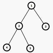
For example, the Euler Tour of this tree would be $$$[(1, 2), (2, 4), (4, 2), (2, 5), (5, 2), (2, 1), (1, 3), (3, 1)]$$$. This is because, while doing a DFS on this tree, you would start off by going from node $$$1$$$ to node $$$2$$$, from node $$$2$$$ to node $$$4$$$, from node $$$4$$$ back to node $$$2$$$, etc.

General Structure

The main idea of Euler Tour Trees is to store the Euler Tour of the tree (hence the name) in some kind of balanced binary search tree (BBST). The split/merge operations offered by BBST's will prove to be extremely useful while implementing the add edge and delete edge operations.

There are a couple of helpful properties in an Euler Tour that we will need:

  • Every edge is stored exactly twice, once for each direction. This implies that there are $$$2(n-1)$$$ edges in a tour.
  • Any cyclic shift of the Euler Tour is still an Euler Tour, but with a different root. This is because the tour is effectively a cycle, and starting a cycle from anywhere is still a cycle.

However, there is one issue that arises: a tree of size $$$1$$$ has an Euler Tour of size $$$0$$$. This is especially an issue when we're using Euler Tour trees, and we're representing a forest of trees (so a degenerate case is very possible). To deal with this, we'll add an extra self-loop $$$(c, c)$$$, for every node $$$c$$$, in the Euler Tour such that the loop occurs right after we enter its corresponding node. This provides a way to support storing values on the nodes as well, not just the edges, when calculating our aggregate operations.

The Operations

Here I'll describe how each of the different operations we're trying to support change the Euler Tour, and how we can reflect those changes in our data structure.

Important note: For all future queries, to locate an edge $$$(a, b)$$$ in the BBST's, you can store a map from "edge" to pointer in the BBST.

Reroot

The reroot operation will be used in the implementation of the future operations, so I will describe it first. The function $$$\text{reroot}(c)$$$ does the following: modify the structure so that it represents the Euler Tour such that you start the DFS at the node $$$c$$$. Recall that any cyclic shift of the Euler Tour is still a valid Euler Tour, so all that's required is finding how much to cyclically shift the edges by (the actual cyclic shift operation can be implemented in $$$\mathcal{O}(\log{} n)$$$ with a BBST). The self-loops that we included make this extra convenient; shifting the tour such that the edge $$$(a, a)$$$ is the first in the list will reroot the tree exactly as intended.

Add Edge

There are three steps when adding an edge between $$$(a, b)$$$:

  1. Call $$$\text{reroot}(a)$$$, so that $$$(a, a)$$$ is the first edge in $$$a$$$'s Euler Tour.
  2. Perform the “reverse” of $$$\text{reroot}(b)$$$, such that $$$(b, b)$$$ is the last edge in $$$b$$$'s Euler Tour.
  3. Merge the two BBST's together (with $$$a$$$'s going before $$$b$$$). Make sure to add the edge $$$(a, b)$$$ in between $$$a$$$ and $$$b$$$ and the edge $$$(b, a)$$$ after $$$b$$$.

Remove Edge

There are 3 steps when removing an edge between $$$(a, b)$$$:

  1. Cyclically shift the edge $$$(a, b)$$$ to the front of the tour.
  2. Remove the edge $$$(a, b)$$$ (now at the front), from the BBST.
  3. Locate and remove the edge $$$(b, a)$$$ from the BBST.

After performing these three operations, the tour will be split into two independent parts (both of which are valid tours of the subtrees)

Subtree Aggregates

To maintain subtree aggregates, one must store subtree aggregates of the values on the edges in the BBST. These will easily get updated while performing the add/remove edge operations. The use of self-loops makes storing weights on vertices extremely simple: just store the values on the self-loop.

Weights can also be updated, by just finding and updating the corresponding edge in the BBST.

Connectivity Checking

This query checks if two nodes $$$a$$$ and $$$b$$$ are in the same component. This can be done simply by just checking if the self loops $$$(a, a)$$$ and $$$(b, b)$$$ are present in the same BBST (e.g. checking if the root of the BBST is the same).

Sample Problems

Thanks for reading the blog! Let me know if you have any suggestions about additions/changes to the blog, or additional sample problems.

Полный текст и комментарии »

  • Проголосовать: нравится
  • +259
  • Проголосовать: не нравится

Автор PurpleCrayon, история, 3 года назад, По-английски

Happy Holidays!

On Dec/24/2021 17:35 (Moscow time) we will host Codeforces Global Round 18.

It is the sixth round of a 2021 series of Codeforces Global Rounds. The rounds are open and rated for everybody.

The presents for this round:

  • 30 best participants get a t-shirt.
  • 20 t-shirts are randomly distributed among those with ranks between 31 and 500, inclusive.

The presents for the 6-round series in 2021:

  • In each round top-100 participants get points according to the table.
  • The final result for each participant is equal to the sum of points he gets in the four rounds he placed the highest.
  • The best 20 participants over all series get sweatshirts and place certificates.

Thanks to XTX, which in 2021 supported the global rounds initiative!

The problems were written and prepared by the hard-working elves Monogon, BledDest, and PurpleCrayon.

We would like to thank the everyone who made this round possible:

You will have 2.5 hours to solve 8 problems.

UPD: The scoring distribution: 250 — 1000 — 1750 — 2250 — 2750 — 3000 — 3750 — 4000

UPD: Editorial is out!

Good luck, have fun, and stay off the naughty list!

Полный текст и комментарии »

  • Проголосовать: нравится
  • +609
  • Проголосовать: не нравится

Автор PurpleCrayon, 3 года назад, По-английски

Hi Codeforces!

I've recently noticed a lack of simulated annealing tutorials, so I decided to make one. It all started when I was trying to "cheese" 1556H - DIY Tree after the contest. In general, simulated annealing is a pretty niche topic, but it can sometimes lend you unintended solutions for very hard problems. It's also very useful in contests like Google Hashcode, where you can add simulated annealing to an already good solution to make it a lot better. Simulated annealing's name and terms are derived from physical annealing, the process of letting metals or glass cool down and harden while removing internal stresses.

An Overview

Simulated Annealing is an approximation algorithm. It's generally useful in problems with low constraints (i.e. $$$n \leq 50$$$ or $$$n \leq 100$$$) where you need to find the minimum/maximum of something over all possible states (and there are usually way too many of them to check). In general, it's good at finding the global maximum/minimum of a function. For the rest of the blog, I'm going to assume that you want to find the minimum of the function (the maximum case is equivalent).

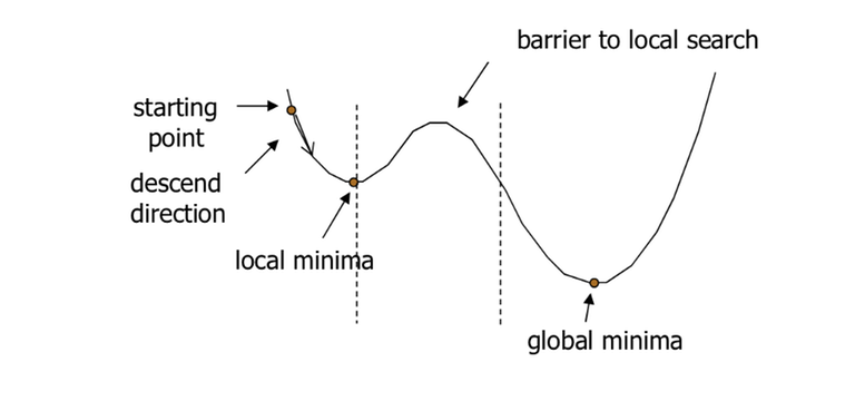
A similar algorithm, that is easier to understand, is called hill-climbing. The way hill-climbing works is that you start with a random state, you find any neighbor of the state, and set the current state to that neighbor if the value of the neighbor state is less than the value of the current state. A "neighbor" of some state is another state that you can get to by applying some small transformation to the previous state (I'll explain more about neighbors in the future). If you look at the image down below, the hill climbing algorithm would look like this:

  1. Start at some random $$$x$$$-value
  2. Change $$$x$$$ by either $$$-1$$$ or $$$+1$$$ (pick the smaller one). In this case $$$x-1$$$ and $$$x+1$$$ are the neighbors of the state.
  3. Repeat until both $$$x-1$$$ and $$$x+1$$$ are larger.

The issue with this algorithm is that it often gets stuck in a local minimum, instead of a global minimum.

Simulated annealing helps fix this issue by sometimes allowing a step to a worse neighbor, which could allow one to reach the global minimum, even if it isn't the same as the local minimum. At each step of the algorithm, you consider some neighboring state and probabilistically decide whether you move to the next state, or keep the current state. You repeat this step until you exhaust the time limit. The crux of simulated annealing is the acceptance probability function, which determines whether you'll take some step or not, depending on the temperature (a value that determines how big of a "bad" step you are going to take). In other words, the higher the temperature, the worse of a state you allow the algorithm to go to (as determined by the acceptance probability function). As iterations progress, temperature gets lower and lower, which causes the algorithm to take smaller and smaller steps until it converges at a global minimum.

Here is some pseudocode:

Let s = random(state) //get's any random valid state
Let best = s
while elapsed_time() <= time_limit:
    Let t = temperature(elapsed_time()/time_limit) //returns temperature given the percent done
    Let next = neighbor(s) //neighbor of a state
    if value(s) < value(best):
        best = s
    if P(value(s), value(next), t) >= random(0, 1): //P -> probability of acceptance function, returns the probability that you'll move to the next state given the value's and the current temperature
        s = next

print(value(best))

In the following sections I'll describe what each function means, and common examples of each function, as well as properties that each function should have.

Neighbor Function

A neighbor function is just a function that takes in a state, and returns a random new state after doing some transformation to the previous state. An important property of the neighbor function is that it doesn't change the answer by too much. Let's start with the example of TSP. An example of a valid neighbor function for TSP is where you swap two the order of two random cities in a state to get a random neighbor of the state. This only affects the values for those two cities, so the answer doesn't change much. Another important property of the "neighbor function" (i.e. how you decide what your neighbors are) is that it should be possible to get any state to any other state in a short number of steps. In the case of TSP, it only takes a linear number of swaps to get from any state to any other state, the hard part of the problem is deciding which swaps to take (which simulated annealing takes care of).

Note: The second condition is important for the accuracy of simulated annealing. For example, simulated annealing wouldn't really work well on a 2-d graph (like the picture I have above — that was purely to demonstrate the existence of local minima), as it takes a lot of steps to move from one end of the graph to the other.

Temperature Function

The temperature function decides how "willing" the algorithm will be to move to a worse state. In other words, if temperature is 0, you'd only ever move to better states (which becomes the hill climbing algorithm). If the temperature is infinity, you'd move to any state, regardless of how good/bad it is. In simulated annealing, you want the temperature to go from something high to something low. Initially, you want to be able to explore the different possible states, so you have a better chance at reaching the global minimum. At the end, when most of the time is used already, you want to keep taking better and better states, hoping that you're already close to the global minimum. There are 3 common temperature reduction rules:

  • $$$t = t \cdot a$$$
  • $$$t = t - a$$$
  • $$$t = \frac{t}{1 + a \cdot t}$$$

Where $$$a$$$ is just some constant that you choose.

The most common one in my experience is the geometric one (the 1st one), where you start with $$$t_0 = 10^9$$$ or $$$t_0 = 10^5$$$ or some other high value and set $$$a = 0.99999$$$.

Acceptance Probability Function

This is the crux of simulated annealing. The acceptance probability function is the function that determines the probability of going from one state to a neighbor state. Let $$$P(old, new, temp)$$$ be the probability from transitioning from a state with value $$$old$$$ to a state with value $$$new$$$ if the current temperature is $$$temp$$$. If we were to use hill climbing, the function would look like this:

def P(old, new, temp):
    if new < old:
        return 1.0
    else:
        return 0.0

This is because you never transition to the next state if it's value is worse. The most common function that's used for simulated annealing is the Metropolis-Hastings Algorithm. This changes the acceptance probability function to:

def P(old, new, temp):
    if new < old:
        return 1.0
    return exp((old-new)/temp)

Now, if the new state is worse you still might transition to it, which makes it more likely that you reach a global minimum. Another important thing to note is that as the temperature decreases, the probability that you transition to a new (worse) state also decreases, which is exactly what we wanted.

Example Problems

Thanks for reading! This was my first tutorial blog, so let me know if there's anything that should be added/changed, I'm always open to suggestions. If you have any other example problems, let me know and I'll add it to the list.

Additionally, thanks to moo. for proofreading the post!

Полный текст и комментарии »

  • Проголосовать: нравится
  • +602
  • Проголосовать: не нравится

Автор PurpleCrayon, история, 3 года назад, По-английски

1541A - Pretty Permutations

Author: PurpleCrayon

Hint
Hint
Hint
Solution

1541B - Pleasant Pairs

Author: PurpleCrayon

Hint
Hint
Solution

1540A - Great Graphs

Author: PurpleCrayon

Hint
Hint
Hint
Solution

1540B - Tree Array

Author: ijxjdjd

Hint
Hint
Hint
Solution

1540C2 - Converging Array (Hard Version)

Author: ijxjdjd

Hint
Hint
Hint
Hint
Solution

1540D - Inverse Inversions

Author: PurpleCrayon

Hint
Hint
Hint
Solution

1540E - Tasty Dishes

Author: ijxjdjd

Hint
Hint
Hint
Hint
Solution

Полный текст и комментарии »

Разбор задач Codeforces Round 728 (Div. 1)
Разбор задач Codeforces Round 728 (Div. 2)
  • Проголосовать: нравится
  • +96
  • Проголосовать: не нравится

Автор PurpleCrayon, история, 3 года назад, По-английски

Hello Codeforces!

ijxjdjd and I are pleased to invite you to participate in Codeforces Round 728 (Div. 1) and Codeforces Round 728 (Div. 2) which will be held on Jun/25/2021 18:35 (Moscow time). Please note the unusual timing. Each division will have 5 problems and 2 hours and 15 minutes to solve them.

We would like to thank:

Read all of the statements carefully, and we hope you enjoy the problems! Wish you high ratings!

UPD: I would also like to thank Roberticey, golions, and 244mhq for testing.

UPD: Here's the score distribution:

Div 1: 500 — 1250 — (1500 + 750) — 3000 — 3500

Div 2: 500 — 1000 — 1500 — 2250 — (2500 + 750)

UPD: The editorial is out!

UPD:

Congratulations to the winners!

Div. 1:

  1. maroonrk
  2. tourist
  3. Radewoosh
  4. LayCurse
  5. NotaMotuaQAQ

Div. 2:

  1. tampa
  2. CF_is_my_GF
  3. Apple_Method
  4. Skybytskyi.Nikita.2
  5. -this-is-obd-

Полный текст и комментарии »

  • Проголосовать: нравится
  • +490
  • Проголосовать: не нравится