


1. Mean↵
-------↵
$$↵
\text{Arithmetic Mean (AM)}: \quad AM = \bar{X} = \frac{\sum_{i=1}^{n} X_i}{n}↵
$$↵
↵
$$↵
\text{Geometric Mean (GM)}: \quad GM = \sqrt[n]{X_1 X_2 \dots X_n} = \left( \prod_{i=1}^{n} X_i \right)^{\frac{1}{n}}↵
$$↵
↵
$$↵
\text{Harmonic Mean (HM)}: \quad HM = \frac{n}{\sum_{i=1}^{n} \frac{1}{X_i}}↵
$$↵
↵
$$↵
\text{AM-GM-HM Inequality}: \quad AM \geq GM \geq HM↵
$$↵
↵
$$↵
\text{Frequency Distribution:}↵
$$↵
$$↵
\begin{array}{|c|c|}↵
\hline↵
\text{Value } X_i & \text{Frequency } f_i \\↵
\hline↵
X_1 & f_1 \\↵
X_2 & f_2 \\↵
... & ... \\↵
X_n & f_n \\↵
\hline↵
\end{array}↵
$$↵
↵
$$↵
\text{Mean for Grouped Data:} \quad \text{Mean} = \frac{\sum_{i=1}^{n} f_i \cdot X_i}{\sum_{i=1}^{n} f_i}↵
$$↵
↵
$$↵
\text{Cumulative Frequency:} \quad \text{Cumulative Frequency} = \sum_{i=1}^{k} f_i↵
$$↵
↵
$$↵
\text{Mean for Continuous Data:} \quad \text{Mean} = \frac{\sum_{i=1}^{n} f_i \cdot M_i}{\sum_{i=1}^{n} f_i}↵
$$↵
↵
2. Median↵
------------------↵
$$↵
\text{Median for Univariate Data:}↵
$$↵
$$↵
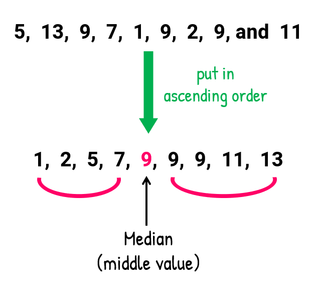
\text{If } n \text{ is odd:} \quad \text{Median} = X_{\left(\frac{n+1}{2}\right)}↵
$$↵
$$↵
\text{If } n \text{ is even:} \quad \text{Median} = \frac{X_{\left(\frac{n}{2}\right)} + X_{\left(\frac{n}{2} + 1\right)}}{2}↵
$$↵
↵
$$↵
\text{Median for Grouped Data:} \quad \text{Median} = L + \left( \frac{\frac{n}{2} - F}{f} \right) \cdot h↵
$$↵
↵
$$↵
\text{Explanation of Terms:}↵
$$↵
$$↵
X \quad \text{: The values in the dataset, ordered from smallest to largest.}↵
$$↵
$$↵
n \quad \text{: Total number of data points or observations.}↵
$$↵
$$↵
L \quad \text{: Lower boundary of the median class in grouped data.}↵
$$↵
$$↵
F \quad \text{: Cumulative frequency before the median class.}↵
$$↵
$$↵
f \quad \text{: Frequency of the median class.}↵
$$↵
$$↵
h \quad \text{: Class width for grouped data.}↵
$$↵
↵
3. Mode↵
------------------↵
$$↵
\text{Mode for Univariate Data:}↵
$$↵
$$↵
\text{Mode} = \text{the most frequent value in the dataset (for unimodal data)}↵
$$↵
$$↵
\text{Mode} = \text{list of most frequent values (for multimodal data)}↵
$$↵
↵
$$↵
\text{Mode for Grouped Data:} \quad \text{Mode} = L + \left( \frac{f_1 - f_0}{(2f_1 - f_0 - f_2)} \right) \cdot h↵
$$↵
↵
$$↵
\text{Explanation of Terms:}↵
$$↵
$$↵
L \quad \text{: Lower boundary of the modal class.}↵
$$↵
$$↵
f_1 \quad \text{: Frequency of the modal class.}↵
$$↵
$$↵
f_0 \quad \text{: Frequency of the class before the modal class.}↵
$$↵
$$↵
f_2 \quad \text{: Frequency of the class after the modal class.}↵
$$↵
$$↵
h \quad \text{: Class width for grouped data.}↵
$$↵
↵
Measure of Location↵
==================↵
A measure which is located in different place in the array is called the measure of location.↵
Median is one kind of measure of location, because median divided whole data set with two parts.↵
↵
Why important measure of location?↵
------------------↵
If you need any number in a data set which is divided the whole data set with in 1:3. It means left side of this set has 1/4 of data and right side has 3/4 data.↵
Most frequently used measure of locations are :↵
1. Median :↵
----------------------------------------------↵
2. Quartile:↵
----------------------------------------------↵
Quartiles divide the data into four equal parts. First Quartile (Q1): The median of the lower half of the data (25% of the data is below Q1).↵
Second Quartile (Q2): The median of the data (50% of the data is below Q2). This is the same as the median.↵
Third Quartile (Q3): The median of the upper half of the data (75% of the data is below Q3).↵
$$↵
\text{Quartiles:}↵
$$↵
$$↵
Q1 \quad \text{(First Quartile)} = \text{Median of the first half of the data.}↵
$$↵
$$↵
Q2 \quad \text{(Second Quartile)} = \text{Median of the dataset.}↵
$$↵
$$↵
Q3 \quad \text{(Third Quartile)} = \text{Median of the second half of the data.}↵
$$↵
↵
3. Decile :↵
---------------------------------------------↵
Deciles divide the data into ten equal parts. Each decile represents 10% of the data.↵
$$↵
\text{Deciles:}↵
$$↵
$$↵
D_n = \frac{n}{100} \cdot (N + 1)↵
$$↵
$$↵
\text{where } n \text{ is the decile number (1 to 9) and } N \text{ is the total number of data points.}↵
$$↵
↵
4. Percentile :↵
--------------------------------------------------↵
Percentiles divide the data into 100 equal parts. Each percentile represents 1% of the data.↵
$$↵
\text{Percentiles:}↵
$$↵
$$↵
P_n = \frac{n}{100} \cdot (N + 1)↵
$$↵
$$↵
\text{where } n \text{ is the percentile number (1 to 100) and } N \text{ is the total number of data points.}↵
$$↵
↵
-------↵
$$↵
\text{Arithmetic Mean (AM)}: \quad AM = \bar{X} = \frac{\sum_{i=1}^{n} X_i}{n}↵
$$↵
↵
$$↵
\text{Geometric Mean (GM)}: \quad GM = \sqrt[n]{X_1 X_2 \dots X_n} = \left( \prod_{i=1}^{n} X_i \right)^{\frac{1}{n}}↵
$$↵
↵
$$↵
\text{Harmonic Mean (HM)}: \quad HM = \frac{n}{\sum_{i=1}^{n} \frac{1}{X_i}}↵
$$↵
↵
$$↵
\text{AM-GM-HM Inequality}: \quad AM \geq GM \geq HM↵
$$↵
↵
$$↵
\text{Frequency Distribution:}↵
$$↵
$$↵
\begin{array}{|c|c|}↵
\hline↵
\text{Value } X_i & \text{Frequency } f_i \\↵
\hline↵
X_1 & f_1 \\↵
X_2 & f_2 \\↵
... & ... \\↵
X_n & f_n \\↵
\hline↵
\end{array}↵
$$↵
↵
$$↵
\text{Mean for Grouped Data:} \quad \text{Mean} = \frac{\sum_{i=1}^{n} f_i \cdot X_i}{\sum_{i=1}^{n} f_i}↵
$$↵
↵
$$↵
\text{Cumulative Frequency:} \quad \text{Cumulative Frequency} = \sum_{i=1}^{k} f_i↵
$$↵
↵
$$↵
\text{Mean for Continuous Data:} \quad \text{Mean} = \frac{\sum_{i=1}^{n} f_i \cdot M_i}{\sum_{i=1}^{n} f_i}↵
$$↵
↵
2. Median↵
------------------↵
$$↵
\text{Median for Univariate Data:}↵
$$↵
$$↵
\text{If } n \text{ is odd:} \quad \text{Median} = X_{\left(\frac{n+1}{2}\right)}↵
$$↵
$$↵
\text{If } n \text{ is even:} \quad \text{Median} = \frac{X_{\left(\frac{n}{2}\right)} + X_{\left(\frac{n}{2} + 1\right)}}{2}↵
$$↵
↵
$$↵
\text{Median for Grouped Data:} \quad \text{Median} = L + \left( \frac{\frac{n}{2} - F}{f} \right) \cdot h↵
$$↵
↵
$$↵
\text{Explanation of Terms:}↵
$$↵
$$↵
X \quad \text{: The values in the dataset, ordered from smallest to largest.}↵
$$↵
$$↵
n \quad \text{: Total number of data points or observations.}↵
$$↵
$$↵
L \quad \text{: Lower boundary of the median class in grouped data.}↵
$$↵
$$↵
F \quad \text{: Cumulative frequency before the median class.}↵
$$↵
$$↵
f \quad \text{: Frequency of the median class.}↵
$$↵
$$↵
h \quad \text{: Class width for grouped data.}↵
$$↵
↵
3. Mode↵
------------------↵
$$↵
\text{Mode for Univariate Data:}↵
$$↵
$$↵
\text{Mode} = \text{the most frequent value in the dataset (for unimodal data)}↵
$$↵
$$↵
\text{Mode} = \text{list of most frequent values (for multimodal data)}↵
$$↵
↵
$$↵
\text{Mode for Grouped Data:} \quad \text{Mode} = L + \left( \frac{f_1 - f_0}{(2f_1 - f_0 - f_2)} \right) \cdot h↵
$$↵
↵
$$↵
\text{Explanation of Terms:}↵
$$↵
$$↵
L \quad \text{: Lower boundary of the modal class.}↵
$$↵
$$↵
f_1 \quad \text{: Frequency of the modal class.}↵
$$↵
$$↵
f_0 \quad \text{: Frequency of the class before the modal class.}↵
$$↵
$$↵
f_2 \quad \text{: Frequency of the class after the modal class.}↵
$$↵
$$↵
h \quad \text{: Class width for grouped data.}↵
$$↵
↵
Measure of Location↵
==================↵
A measure which is located in different place in the array is called the measure of location.↵
Median is one kind of measure of location, because median divided whole data set with two parts.↵
↵
Why important measure of location?↵
------------------↵
If you need any number in a data set which is divided the whole data set with in 1:3. It means left side of this set has 1/4 of data and right side has 3/4 data.↵
Most frequently used measure of locations are :↵
1. Median :↵
----------------------------------------------↵
2. Quartile:↵
----------------------------------------------↵
Quartiles divide the data into four equal parts. First Quartile (Q1): The median of the lower half of the data (25% of the data is below Q1).↵
Second Quartile (Q2): The median of the data (50% of the data is below Q2). This is the same as the median.↵
Third Quartile (Q3): The median of the upper half of the data (75% of the data is below Q3).↵
$$↵
\text{Quartiles:}↵
$$↵
$$↵
Q1 \quad \text{(First Quartile)} = \text{Median of the first half of the data.}↵
$$↵
$$↵
Q2 \quad \text{(Second Quartile)} = \text{Median of the dataset.}↵
$$↵
$$↵
Q3 \quad \text{(Third Quartile)} = \text{Median of the second half of the data.}↵
$$↵
↵
3. Decile :↵
---------------------------------------------↵
Deciles divide the data into ten equal parts. Each decile represents 10% of the data.↵
$$↵
\text{Deciles:}↵
$$↵
$$↵
D_n = \frac{n}{100} \cdot (N + 1)↵
$$↵
$$↵
\text{where } n \text{ is the decile number (1 to 9) and } N \text{ is the total number of data points.}↵
$$↵
↵
4. Percentile :↵
--------------------------------------------------↵
Percentiles divide the data into 100 equal parts. Each percentile represents 1% of the data.↵
$$↵
\text{Percentiles:}↵
$$↵
$$↵
P_n = \frac{n}{100} \cdot (N + 1)↵
$$↵
$$↵
\text{where } n \text{ is the percentile number (1 to 100) and } N \text{ is the total number of data points.}↵
$$↵
↵

