


For a contest I was one of the main contributors to, I came up with the following problem:
Problem
There are $$$n$$$ points on a circle numbered 0 to $$$n-1$$$. You are given $$$k$$$ pairs $$$(x_i, y_i)$$$ where $$$x_i\neq y_i$$$. For the $$$i$$$-th pair, you need to choose $$$S_i$$$ to be $$$[x_i, y_i)$$$ or $$$[y_i, x_i)$$$. This is a cyclic range, meaning if $$$a \gt b$$$, then $$$[a, b) = {a \dots n-1, 0 \dots b-1}$$$.
We say an unordered pair $$$(i, j)$$$ (possibly $$$i=j$$$) is connected if there exists some $$$l$$$ such that $$$i \in S_l$$$ and $$$j \in S_l$$$. Note that although I call it connected, I don't mean it to be a transitive property.
Let $$$S$$$ be the set of connected unordered pairs. For each unordered pair $$$(i, j)$$$, you are given a nonnegative cost $$$C[i][j]$$$. The cost of $$$S$$$ is defined to be the sum of the costs of all unordered pairs in $$$S$$$. The task is to find the minimal possible cost of $$$S$$$, given the cost matrix $$$C$$$ and the $$$k$$$ pairs.
I found the problem quite difficult, although the final structure feels deceptively simple in hindsight. Below is a description of the solution my friends and I came up with, which has a time complexity of $$$\mathcal{O}(n^5)$$$. I encourage you to try to solve the problem yourselves first!
Solution
Let's start by solving a specific case of the problem: $$$C[i][j] = 1$$$, and every unordered pair $$${x_i,y_i}$$$ appears exactly once in the input, thus $$$k = \binom{n}{2}$$$. The answer should depend only on $$$n$$$.
We can think about the problem in the following way: We have a bit matrix $$$A$$$ of size $$$n \times n$$$ initially filled with 0s, and for every given pair $$$(x, y)$$$, we need to color either $$$[x, y)^2$$$ or $$$[y, x)^2$$$. We want to maximize the number of 0s at the end of the process (counting only up to the main diagonal).
A brute-force search for small values of $$$n$$$ suggests that the maximal number of 0s is exactly $$$n$$$, and every optimal solution will have a very specific structure. The set of 0s is always a right-up path starting at $$$(n - 1 - a, 0)$$$ and ending at $$$(n - 1, b)$$$ of length $$$n$$$ (containing $$$n$$$ points, i.e. $$$a + b + 1 = n$$$).

We can see why it has to be a right-up path: there can't be two 0s on the same $$$x+y$$$ diagonal because between them there will be a "barrier". Whichever interval we choose, all 0s must remain on the same side of that barrier:

In this picture, we need to choose to color either the blue area or the red area. This puts a barrier (the green barrier) between the two yellow points. For any 2 points with the same $$$x+y$$$ value there exists such a barrier.
But why must it be of length $$$n$$$? For that, we need to expand our definition of a "diagonal".
Let's try to understand the topology we are working with. $$$(n, x)$$$ is identified with $$$(0, x)$$$, and $$$(x, n)$$$ is identified with $$$(x, 0)$$$ (in the sense that after point $$$n-1$$$ on the circle comes point 0). This quotient is famously known to be a torus. But we also have another condition: $$$(x, y)$$$ is identified with $$$(y, x)$$$ because the pairs are unordered. This turns our topology into a Möbius band. Here is a fundamental polygon calculation that shows this is the case:

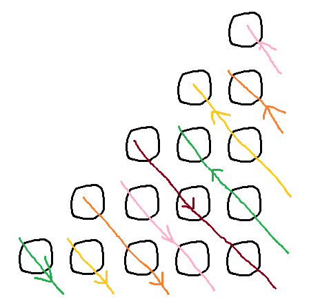
Arrows of the same color are identified in the indicated direction; the sequence of cuts and gluings converts the quotient into the standard fundamental polygon of a Möbius band.
The "columns" of this Möbius band are exactly the diagonals we looked for! We have $$$n$$$ diagonals, and each of them is the set of points $$$(x, y)$$$ with the same $$$(x + y) \pmod n$$$.
Every one of the $$$k$$$ pairs lands on one of the $$$n$$$ diagonals and forces us to choose a side. Because in this case we are given all $$$\binom{n}{2}$$$ pairs, there can be at most one 0 on each of the $$$n$$$ diagonals, so the number of 0s is at most $$$n$$$. (The maximum number of 0s, as it turns out, is exactly $$$n$$$, the matching construction will follow from the claims below).
Let's try to generalize this to a full solution. How does our Möbius band transformation look? Every point is adjacent to up two points in every neighboring diagonal, giving us a hex-like grid which looks a bit different depending on the parity of $$$n$$$. Every one of the given $$$k$$$ pairs serves as a barrier on one of the diagonals.
For example, for the following input:
We will get the following structure:
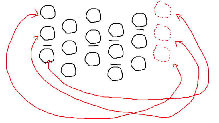
We call a set $$$\mathcal{L}$$$ of points a valid loop if:
- It forms a contiguous segment in every column of the Möbius band.
- Every two neighboring columns connect nicely (see picture). Concretely, the respective endpoints of the neighboring columns should be adjacent in the hex grid.
- It contains no barriers inside its area.
We define the weight of $$$\mathcal{L}$$$ as the sum of the costs of all points in it. I argue that the answer is the sum of the costs of all pairs minus the maximum weight of a valid loop. So for the example input above, the maximum valid loop will be:

Here the points outside the black region form the valid loop. This has weight 8, so the answer is $$$\binom{6}{2} - 8 = 7$$$.
Proof
Direction 1: Every valid loop $$$\mathcal{L}$$$ is contained in the disconnected set of some assignment
Proof: For each barrier, choose the side that avoids $$$\mathcal{L}$$$ in the barrier's column. We just need to show that this also avoids $$$\mathcal{L}$$$ in every other column. Property 2 guarantees this: as we move between neighboring columns, the endpoints of $$$\mathcal{L}$$$ can move only along adjacent grid edges, which is exactly the rate at which either side of a barrier expands.
Direction 2: Every set of disconnected pairs of some assignment can be extended to a valid loop
Proof: If we look at a range in one column, we can extend the set in a way such that all points in its "shrinking" are also contained in the set.

Explanation: Assume the range in the left column is contained in the set of disconnect pairs. We show that we can obtain all the non black points in the picture. Assume for the sake of contradiction that there is a barrier (the green barrier) contained in the white area. Then one of its sides, the blue side or the red side, contains a point in the original range, contradicting the assumption that the original range consists of disconnected pairs under some assignment.
This shows that, once every column contains at least one disconnected pair, the disconnected set can be extended to satisfy the conditions of a valid loop.
So let's assume there are two diagonals (I am talking now about diagonals in the original matrix representation) with some nonempty range of disconnected pairs on them, and every diagonal between them has no disconnected pairs on it. Then we can extend the set of disconnected pairs in the following way:
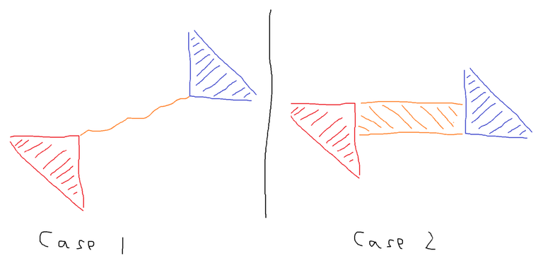
Explanation: In case 1, we shrink the red range on the left to a single point, and do the same thing for the blue range on the right but in the opposite direction. We connect these two points with some right-up path. In case 2, we do a similar thing except that we fill the area between the two points with a rectangle. Any barrier in the orange region will have one side contain a point from the original red range, and the other side will contain a point from the original blue range, contradicting our assumption. There are a couple more cases that you can check if you want but it's all really the same thing. The point is that if there are two disconnected pairs on the same row (in the original matrix representation) then everything between them also has to be disconnected.
Note that because all costs are nonnegative, extending the set of disconnected pairs can only increase its total weight.
Algorithm
We now do the most naive algorithm possible for calculating the maximum weight of a valid loop. Define dp[s,e][l,r][i] as the maximum weight of a valid walk starting in column 0 with the range $$$[s, e]$$$ that ends in column $$$i$$$ with the range $$$[l, r]$$$. We then take the maximum over all walks that connect at the ends (this roughly corresponds to dp[s,e][n/2-e, n/2-s][n-1]). Each state considers only $$$\mathcal{O}(1)$$$ previous states, so the time complexity is $$$\mathcal{O}(n^5)$$$. For exact details on the DP transitions, see the implementation.
You can also do DP directly on the original table representation (a valid loop is a right-up band going around the matrix with $$$(n, x)\sim(x, 0)$$$), but I think this approach is more elegant.
Can you solve this problem in $$$o(n^5)$$$?
The reason I am writing this blog is because I am frustrated that I wasn't able to reduce the time complexity down from $$$\mathcal{O}(n^5)$$$. It feels very disappointing that we made all those claims about the geometry of the problem, and then once we understood it, we did the most naive thing we could have done.
I have spent a lot of time trying to reduce the time complexity, but everything I tried failed. For example, attempts on supermodularity properties (which this DP does have, but precisely in a way that doesn't help us) didn't work out.
It would be amazing if someone could optimize the algorithm. It doesn't feel quite right that this is the best we can do.
More Thoughts
We can try to extend the problem in a couple of different directions:
- Negative costs: What if the costs could have been negative? I think there is a solution in $$$\mathcal{O}(n^7)$$$ or $$$\mathcal{O}(n^8)$$$ but this doesn't sound too interesting.
- Higher dimensions: What if we increased the dimension of the problem? Instead of counting pairs, we would count $$$d$$$-tuples (or a weighted combination of them). The topology of this is quite interesting. For odd $$$d$$$, we get a $$$d$$$-dimensional analogue of the solid torus. For even $$$d$$$ we get the twisted, non-orientable version of this. Concretely, for odd $$$d$$$ we have $$$SP^d(S^1) \cong S^1 \times \Delta^{d-1}$$$ and for even $$$d$$$ we have $$$SP^d(S^1) \cong S^1 \tilde{\times} \Delta^{d-1}$$$ where $$$\tilde{\times}$$$ denotes the non-trivial (twisted) product over $$$S^1$$$. For example, for $$$d=3$$$ we get the solid torus. I think I can use this to make an algorithm with time complexity somewhere between $$$\mathcal{O}(n^{11})$$$ and $$$\mathcal{O}(n^{15})$$$ for the $$$d=3$$$ case, although I am not quite sure about that. It makes a lot of sense to conjecture that there is an algorithm of time complexity $$$\mathcal{O}(n^{f(d)})$$$ for every $$$d$$$. My intuition says that as we get to higher dimensions, the barriers get sparser, so the problem may become easier. Does there exist a polynomial algorithm with $$$d$$$ as part of the input (with the cost function defined somehow implicitly, for example an interesting case is a positive linear combination)?
- Infinite dimensions: What if we take this to the limit? A generalization worth considering is counting connected subsets, again with the cost function defined implicitly. I didn't give much thought to this. Topologically, I am not quite sure what we have. I have some ideas, but I don't want to be imprecise.
- Different choices: What if instead of choosing between $$$[x, y)$$$ we are given a sequence $$$a_0 \lt \dots \lt a_{l-1}$$$ and we need to choose some $$$[a_i, a_{(i+1)\bmod l})$$$? I think we are stepping into NP-hard territory, but I am ready to be surprised.
Special thanks to DnlPrs809 for thinking with me about the problem and reviewing the blog!
Thank you for reading! I hope you found the question(s) interesting. Hope you liked my Microsoft Paint skills :)


